Length of a Vector
Determinant of Covariance Matrix
|Σ| = det(Σ)
Test Vector
Length of a Vector
|x| = sqrt( Σx2)
By the Pythagorean Theorem:
Correlation
The correlation between any two vectors is

where θ is the angle between the two vectors.
Covariance Matrix
The sample covariance matrix,
where each xij is the deviation score of the ith person on the jth test.
Determinant
The determinant of the covariance matrix is
Area = base * height
K Groups
Consider k groups with matrices X1, X2, ..., Xk each with p variables.
Wilks' Lambda
Where W is the pooled within Deviation SSCP derived separately from each Xi
W = S1 + S2 + ... + Sk
T is the total Deviation SSCP computed from X.
Using covariance matrices:
Univariate Case
When p = 1,
It must be the case that
Thus in the univariate case Λ and F are inversely related. This relation also holds in the multivariate case as well.
F Approximation
An F approximation for Λ is
with df = p(k-1) and ms - p(k-1)/2 + 1, where
Special Note Concerning s
If either the numerator or the deminator of s = 0, then set s = 1.
Exact F
Three Group Example
Employees in three job categories (c1 Passenger Agents; c2 Mechanics; c3 Operations Control) of an airline company were administered an activity preference questionnaire consisting of three bipolar scales: y1 outdoor-indoor preferences; y2 convivial-solitary preferences; y3 conservative-liberal preferences.
Given matrices W and T, test the hypothesis that the three group centroids are significantly diffenent from one another.
Stata Matrix Program
scalar k = 3
scalar n1 = 85
scalar n2 = 93
scalar n3 = 66

matrix w = (3967.8301, 351.6142, 76.6342 \   ///
            351.6142, 4406.2517, 235.4365 \  ///
             76.6342, 235.4365, 2683.3164)

matrix t = (5540.5742, -421.4364, 350.2556 \ ///
            -421.4364, 7295.571, -1170.559 \ ///
             350.2556, -1170.559, 3374.9232)

scalar p = rowsof(w)
scalar dw = det(w)
scalar dt = det(t)
scalar lambda = dw/dt
display "lambda = " lambda

scalar n = n1+n2+n3
scalar c = (n-p-2)/p
scalar f = (1-sqrt(lambda))/sqrt(lambda)*c
display "F = " f

scalar df1 = 2*p
scalar df2 = 2*(n-p-2)
display  "df1 = " df1 "    df2 = " df2
Stata ExampleExample with significant multivariate but no significant univariates.
Plot of Means
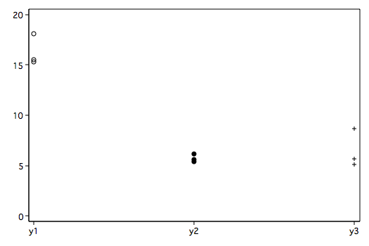
input group y1 y2 y3
1 19.6 5.15 9.5
1 15.4 5.75 9.1
1 22.3 4.35 3.3
1 24.3 7.55 5.0
1 22.5 8.50 6.0
1 20.5 10.25 5.0
1 14.1 5.95 18.8
1 13.0 6.30 16.5
1 14.1 5.45 8.9
1 16.7 3.75 6.0
1 16.8 5.10 7.4
2 17.1 9.00 7.5
2 15.7 5.30 8.5
2 14.9 9.85 6.0
2 19.7 3.60 2.9
2 17.2 4.05 0.2
2 16.0 4.40 2.6
2 12.8 7.15 7.0
2 13.6 7.25 3.2
2 14.2 5.30 6.2
2 13.1 3.10 5.5
2 16.5 2.40 6.6
3 16.0 4.55 2.9
3 12.5 2.65 0.7
3 18.5 6.50 5.3
3 19.2 4.85 8.3
3 12.0 8.75 9.0
3 13.0 5.20 10.3
3 11.9 4.75 8.5
3 12.0 5.85 9.5
3 19.8 2.85 2.3
3 16.5 6.55 3.3
3 17.4 6.60 1.9
end

tabstat y1 y2 y3, by(group) stat(n mean sd var) col(stat)

Summary for variables: y1 y2 y3
     by categories of: group

   group |         N      mean        sd  variance
---------+----------------------------------------
       1 |        11  18.11818  3.903797  15.23963
         |        11  6.190909  1.899713  3.608909
         |        11  8.681818  4.863089  23.64963
---------+----------------------------------------
       2 |        11  15.52727  2.075616  4.308182
         |        11  5.581818  2.434263  5.925637
         |        11  5.109091  2.531187  6.406909
---------+----------------------------------------
       3 |        11  15.34545  3.138268  9.848727
         |        11  5.372727  1.759029  3.094182
         |        11  5.636364  3.546907  12.58055
---------+----------------------------------------
   Total |        33   16.3303  3.292461   10.8403
         |        33  5.715152  2.017598  4.070701
         |        33  6.475758  3.985131  15.88127
--------------------------------------------------

manova y1 y2 y3 = group

                           Number of obs =      33

                           W = Wilks' lambda      L = Lawley-Hotelling trace
                           P = Pillai's trace     R = Roy's largest root

                  Source |  Statistic     df   F(df1,    df2) =   F   Prob>F
              -----------+--------------------------------------------------
                   group | W   0.5258      2     6.0    56.0     3.54 0.0049 e
                         | P   0.4767            6.0    58.0     3.02 0.0122 a
                         | L   0.8972            6.0    54.0     4.04 0.0021 a
                         | R   0.8920            3.0    29.0     8.62 0.0003 u
                         |--------------------------------------------------
                Residual |                30
              -----------+--------------------------------------------------
                   Total |                32
              --------------------------------------------------------------
                           e = exact, a = approximate, u = upper bound on F
Univariate Analyses for Comparisons
anova y1 group

                           Number of obs =      33     R-squared     =  0.1526
                           Root MSE      = 3.13031     Adj R-squared =  0.0961

                  Source |  Partial SS    df       MS           F     Prob > F
              -----------+----------------------------------------------------
                   Model |  52.9242378     2  26.4621189       2.70     0.0835
                         |
                   group |  52.9242378     2  26.4621189       2.70     0.0835
                         |
                Residual |  293.965442    30  9.79884808
              -----------+----------------------------------------------------
                   Total |   346.88968    32  10.8403025

anova y2 group

                           Number of obs =      33     R-squared     =  0.0305
                           Root MSE      = 2.05173     Adj R-squared = -0.0341

                  Source |  Partial SS    df       MS           F     Prob > F
              -----------+----------------------------------------------------
                   Model |  3.97515121     2   1.9875756       0.47     0.6282
                         |
                   group |  3.97515121     2   1.9875756       0.47     0.6282
                         |
                Residual |  126.287277    30  4.20957589
              -----------+----------------------------------------------------
                   Total |  130.262428    32  4.07070087

anova y3 group

                           Number of obs =      33     R-squared     =  0.1610
                           Root MSE      = 3.76993     Adj R-squared =  0.1051

                  Source |  Partial SS    df       MS           F     Prob > F
              -----------+----------------------------------------------------
                   Model |  81.8296936     2  40.9148468       2.88     0.0718
                         |
                   group |  81.8296936     2  40.9148468       2.88     0.0718
                         |
                Residual |  426.370896    30  14.2123632
              -----------+----------------------------------------------------
                   Total |   508.20059    32  15.8812684
Multivariate Post-hoc Comparisons
manovatest, showorder

 Order of columns in the design matrix
      1: _cons
      2: (group==1)
      3: (group==2)
      4: (group==3)

mat d1 = (0,1,-1,0)
mat d2 = (0,1,0,-1)
mat d3 = (0,0,1,-1)

manovatest, test(d1)

 Test constraint
 (1)    group[1] - group[2] = 0

                           W = Wilks' lambda      L = Lawley-Hotelling trace
                           P = Pillai's trace     R = Roy's largest root

                  Source |  Statistic     df   F(df1,    df2) =   F   Prob>F
              -----------+--------------------------------------------------
              manovatest | W   0.5875      1     3.0    28.0     6.55 0.0017 e
                         | P   0.4125            3.0    28.0     6.55 0.0017 e
                         | L   0.7020            3.0    28.0     6.55 0.0017 e
                         | R   0.7020            3.0    28.0     6.55 0.0017 e
                         |--------------------------------------------------
                Residual |                30
              --------------------------------------------------------------
                           e = exact, a = approximate, u = upper bound on F

manovatest, test(d2)

 Test constraint
 (1)    group[1] - group[3] = 0

                           W = Wilks' lambda      L = Lawley-Hotelling trace
                           P = Pillai's trace     R = Roy's largest root

                  Source |  Statistic     df   F(df1,    df2) =   F   Prob>F
              -----------+--------------------------------------------------
              manovatest | W   0.6109      1     3.0    28.0     5.95 0.0029 e
                         | P   0.3891            3.0    28.0     5.95 0.0029 e
                         | L   0.6370            3.0    28.0     5.95 0.0029 e
                         | R   0.6370            3.0    28.0     5.95 0.0029 e
                         |--------------------------------------------------
                Residual |                30
              --------------------------------------------------------------
                           e = exact, a = approximate, u = upper bound on F

manovatest, test(d3)

 Test constraint
 (1)    group[2] - group[3] = 0

                           W = Wilks' lambda      L = Lawley-Hotelling trace
                           P = Pillai's trace     R = Roy's largest root

                  Source |  Statistic     df   F(df1,    df2) =   F   Prob>F
              -----------+--------------------------------------------------
              manovatest | W   0.9932      1     3.0    28.0     0.06 0.9785 e
                         | P   0.0068            3.0    28.0     0.06 0.9785 e
                         | L   0.0068            3.0    28.0     0.06 0.9785 e
                         | R   0.0068            3.0    28.0     0.06 0.9785 e
                         |--------------------------------------------------
                Residual |                30
              --------------------------------------------------------------
                           e = exact, a = approximate, u = upper bound on F
To control for the conceptual error rate, you can divide the p-values by the number
of comparisons for a Bonferroni adjustment.Multivariate Strength of Association
Given a sufficiently large sample almost any difference can be statistically significant.
In the univariate case the correlation ratio measures strength of association,
is a direct multivariate generalization of the correlation ratio. Unfortunately, it tends to be positively biased, grossly overestimating the strength of association.
A better estimate of strength of association is
which is also positively biased, leading to a corrected version.

which is nearly unbiased.
In the example above:
Simultaneous Confidence Intervals
simulci y1 y2 y3, by(group) cv(.325)  /* findit simulci */

s=2  m=0  n=13 cv= .325

group variable:   group

                                    pairwise simultaneous
comparison           difference      confidence intervals
dv: y1
group 1 vs group 2        2.591*        0.212         4.970
group 1 vs group 3        2.773*        0.393         5.152
group 2 vs group 3        0.182        -2.198         2.561

dv: y2
group 1 vs group 2        0.609        -0.950         2.169
group 1 vs group 3        0.818        -0.741         2.378
group 2 vs group 3        0.209        -1.350         1.769

dv: y3
group 1 vs group 2        3.573*        0.707         6.438
group 1 vs group 3        3.045*        0.180         5.911
group 2 vs group 3       -0.527        -3.393         2.338
Where cv is the critical value taken from the Heck charts (see Morrison, 2005 or
charts).
Where,Why can't I just do a bunch of univariate anovas instead of a manova?
The answer is you can. Its not the correct analysis but you could do it. There are a couple of problems with running a separate univariate anovas. One is the the analyses are not independent of one another because the response variables are, most likely, correlated with one another. Therefore, an analysis with one response variable is not independent with one done a different one, that is, the analyses do not necessarily provide different or unique information.
Manova uses information from each of the response variables taking into account their correlated nature. This is one reason why multivariate tests are more powerful than their univariate counterparts, they have more information to work with.
But, even if the response variables were completely independent of one another, a multivariate test would be preferred because problems with the conceptual error rate. When response variables are independent and each anova is tested at α, the the probability of making at least one Type I error in n anovas is 1 - (1 - α)n.
The table below gives the probability of making at least one type I error for four different numbers of anovas:
 n    probability
 3      .1426
 5      .2262
10      .4013
15      .5367
Conceptual Error Rates
And once you factor in any post-hoc comparisons in each anova, you have to watch out for problems with the conceptual error rate, in particular the probability that at least one test is significant by chance alone.
Multivariate Course Page
Phil Ender, 23oct07, 17jul07, 25oct05, 20may02, 29jan98