The General Linear Model
The General Linear Model provides a framework for analyzing arbitrary univariate or multivariate regression, anova and ancova models. In Stata the manova command is used to fit general linear models, SAS calls the procedure proc glm.
H = A'(CB)'(C(X'X)-1C')-1(CB)A
E = A'(Y'Y - B'(X'X)B)A
where B = (X'X)-1X'Y
The A matrix operates on the dependent variables while the C matrix operates on the independent variables.
Consider the Design
manova y1 y2 = a b;
with a having 3 levels and b having 2 levels, the parameter vector is:
To test all the pairwise differences among the levels of a, use the following C matrices in the manovatest command:
C1 = (0, 1, -1,  0, 0, 0)
C2 = (0, 1,  0, -1, 0, 0)
C3 = (0, 0,  1, -1, 0, 0)
     (μ  α1  α2  α3 β1 β2)
manova y1 y2 = a b
manovatest , test(C1)
manovatest , test(C2)
manovatest , test(C3)
Dependent Variables
The A matrix is also used in the manovatest command, for example, consider the difference in two dependent variables:
A = (1, -1)
manova y1 y2 = a b
manovatest a,  ytransform(A)
Memory Test
Remember the Linear model form Ed230B/C
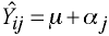
Yij = μ + αj + εij

The effect parameter: αj = μj - μ
Coding
Using dummy coding for two groups
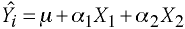
X0 = 1, X1 = 1 or 0, and X2 = 0 or 1
Which yields two equations in three unknowns. The system is rank deficient with no unique solution.
Let α1 = μ1 - μ and α2 = μ2 - μ
Hence: α1 + α2 = μ1 + μ2 - 2μ
and since 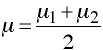
thus, 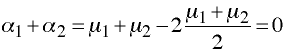
By constraining α1 + α2 = 0 leads to a set of equations which are not deficient rank.
Matrix Form
In matrix form
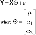
which is deficient rank.
Reparameterization
A more desireable way to manage deficient rank is to reparameterize, that is, choose to estimate two linear combinations of the parameters of Θ.
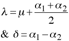
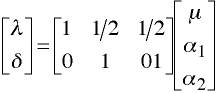
Let
Matrix Form
Thus,
![]()
Where C is the contrast matrix.
now Y = KΘ* + ε in which
K = (XC')(CC')-1. Thus
![]()
Assignment 9 Notes
For the purposes of Assignment 9, we will not use the two stage estimation process. By using our standard orthogonal coding we will take care of the reparameterization.
Here are the formulas for H and E without the A matrix:
B = (X'X)-1X'Y
H = (CB)'(C(X'X)-1C')-1(CB)
E = (Y'Y - B'(X'X)B)
To do Assignment 9, you will need to compute E once and compute H three times. The three H matrices are, one each for, a main effects, b main effects and a*b interaction.
Alternative GLM Formulation
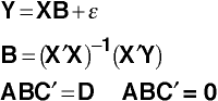
where A operates on coefficients. B is the matrix of regression coefficients. C operates on dependent variables and D operates on H0's.
SSCP Matrices
Total  =  Model + Residual
ST     =   SM   +    SR
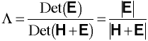
Wilks' Lambda
Rao's F Approximation
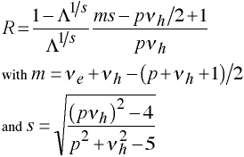
Special Note Concerning s
If either the numerator or the dominator of s = 0 set s = 1.
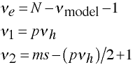
Degrees of Freedom
Consider the Design
| B | ||||
|---|---|---|---|---|
| b1 | b2 | b3 | ||
| y1 y2 | y1 y2 | y1 y2 | ||
| A | a1 | 32 16 29 11 | 34 17 30 13 | 33 18 30 15 |
| a2 | 34 19 27 10 | 33 15 32 12 | 31 17 31 14 | |
| a3 | 33 15 26 12 | 32 16 31 11 | 32 16 32 13 | |
input y1 y2 a b
32 16 1 1
29 11 1 1
34 17 1 2
30 13 1 2
33 18 1 3
30 15 1 3
34 19 2 1
27 10 2 1
33 15 2 2
32 12 2 2
31 17 2 3
31 14 2 3
33 15 3 1
26 12 3 1
32 16 3 2
31 11 3 2
32 16 3 3
32 13 3 3
end

manova y1 y2 = a b a*b

                           Number of obs =      18

                           W = Wilks' lambda      L = Lawley-Hotelling trace
                           P = Pillai's trace     R = Roy's largest root

                  Source |  Statistic     df   F(df1,    df2) =   F   Prob>F
              -----------+--------------------------------------------------
                   Model | W   0.4623      8    16.0    16.0     0.47 0.9287 e
                         | P   0.5934           16.0    18.0     0.47 0.9299 a
                         | L   1.0429           16.0    14.0     0.46 0.9328 a
                         | R   0.9108            8.0     9.0     1.02 0.4808 u
                         |--------------------------------------------------
                Residual |                 9
              -----------+--------------------------------------------------
                       a | W   0.9296      2     4.0    16.0     0.15 0.9609 e
                         | P   0.0705            4.0    18.0     0.16 0.9537 a
                         | L   0.0755            4.0    14.0     0.13 0.9680 a
                         | R   0.0733            2.0     9.0     0.33 0.7273 u
                         |--------------------------------------------------
                       b | W   0.6079      2     4.0    16.0     1.13 0.3772 e
                         | P   0.4203            4.0    18.0     1.20 0.3459 a
                         | L   0.5986            4.0    14.0     1.05 0.4179 a
                         | R   0.5071            2.0     9.0     2.28 0.1579 u
                         |--------------------------------------------------
                     a*b | W   0.7281      4     8.0    16.0     0.34 0.9351 e
                         | P   0.2753            8.0    18.0     0.36 0.9288 a
                         | L   0.3688            8.0    14.0     0.32 0.9437 a
                         | R   0.3555            4.0     9.0     0.80 0.5547 u
                         |--------------------------------------------------
                Residual |                 9
              -----------+--------------------------------------------------
                   Total |                17
              --------------------------------------------------------------
                           e = exact, a = approximate, u = upper bound on F
GLM Matrices
The Y matrix has 18 rows and two columns. One row for each subject in the design and one column for each dependent variable.
#delimit ;
mat y = (
32,16\
29,11\
34,17\
30,13\
33,18\
30,15\
34,19\
27,10\
33,15\
32,12\
31,17\
31,14\
33,15\
26,12\
32,16\
31,11\
32,16\
32,13);
#delimit cr

mata; y = (32,16\29,11\34,17\30,13\33,18\30,15\34,19\27,10\33,15\32,12\31,17\31,14\33,15\26,12\32,16\31,11\32,16\32,13)
The X matrix contains the orthogonally coded independent variables for
classifying the observations into a 3x3 factorial design. The columns of the X matrix are:
x0 - grand mean
x1, x2 - A main effect
x3, x4 - B main effect
x5, x6, x7, x8 - A*B interaction
#delimit ;
mat x = (
1,  1,  1,  1,  1,  1,  1,  1,  1\
1,  1,  1,  1,  1,  1,  1,  1,  1\
1,  1,  1, -1,  1, -1,  1, -1,  1\
1,  1,  1, -1,  1, -1,  1, -1,  1\
1,  1,  1,  0, -2,  0, -2,  0, -2\
1,  1,  1,  0, -2,  0, -2,  0, -2\
1, -1,  1,  1,  1, -1, -1,  1,  1\
1, -1,  1,  1,  1, -1, -1,  1,  1\
1, -1,  1, -1,  1,  1, -1, -1,  1\
1, -1,  1, -1,  1,  1, -1, -1,  1\
1, -1,  1,  0, -2,  0,  2,  0, -2\
1, -1,  1,  0, -2,  0,  2,  0, -2\
1,  0, -2,  1,  1,  0,  0, -2, -2\
1,  0, -2,  1,  1,  0,  0, -2, -2\
1,  0, -2, -1,  1,  0,  0,  2, -2\
1,  0, -2, -1,  1,  0,  0,  2, -2\
1,  0, -2,  0, -2,  0,  0,  0,  4\
1,  0, -2,  0, -2,  0,  0,  0,  4);
#delimit cr

mata; x = (1,  1,  1,  1,  1,  1,  1,  1,  1\1,  1,  1,  1,  1,  1,  1,  1,  1\1,  1,  1, -1,  1, -1,  1, -1,  1\1,  1,  1, -1,  1, -1,  1, -1,  1\1,  1,  1,  0, -2,  0, -2,  0, -2\1,  1,  1,  0, -2,  0, -2,  0, -2\1, -1,  1,  1,  1, -1, -1,  1,  1\1, -1,  1,  1,  1, -1, -1,  1,  1\1, -1,  1, -1,  1,  1, -1, -1,  1\1, -1,  1, -1,  1,  1, -1, -1,  1\1, -1,  1,  0, -2,  0,  2,  0, -2\1, -1,  1,  0, -2,  0,  2,  0, -2\1,  0, -2,  1,  1,  0,  0, -2, -2\1,  0, -2,  1,  1,  0,  0, -2, -2\1,  0, -2, -1,  1,  0,  0,  2, -2\1,  0, -2, -1,  1,  0,  0,  2, -2\1,  0, -2,  0, -2,  0,  0,  0,  4\1,  0, -2,  0, -2,  0,  0,  0,  4)
L Matrices
You will need three L matrices. One each for A main effect, B main effect, and A*B interaction.
#delimit ;
mat l = (
0, 1, 0, 0, 0, 0, 0, 0, 0\
0, 0, 1, 0, 0, 0, 0, 0, 0);
#delimit cr

mata; l = (0, 1, 0, 0, 0, 0, 0, 0, 0\0, 0, 1, 0, 0, 0, 0, 0, 0)
#delimit ;
mat l = (
0, 0, 0, 1, 0, 0, 0, 0, 0\
0, 0, 0, 0, 1, 0, 0, 0, 0);
#delimit cr

mata; l = (0, 0, 0, 1, 0, 0, 0, 0, 0\0, 0, 0, 0, 1, 0, 0, 0, 0)
#delimit ;
mat l = (
0, 0, 0, 0, 0, 1, 0, 0, 0\
0, 0, 0, 0, 0, 0, 1, 0, 0\
0, 0, 0, 0, 0, 0, 0, 1, 0\
0, 0, 0, 0, 0, 0, 0, 0, 1);
#delimit cr

mata; l = (0, 0, 0, 0, 0, 1, 0, 0, 0\0, 0, 0, 0, 0, 0, 1, 0, 0\0, 0, 0, 0, 0, 0, 0, 1, 0\0, 0, 0, 0, 0, 0, 0, 0, 1)
GLM Formulas
B = (X'X)-1X'Y
H = (LB)'(L(X'X)-1L')-1(LB)
E = (Y'Y - B'(X'X)B)
Λ = det(E)/det(H + E)
Some Matrix Code
Stata                                    Mata
mat xx = x'*x                            xx = x'*x
mat b = syminv(xx)*x'*y                  b  = invsym(xx)*x'*y
mat e = y'*y - b'*xx*b                   e  = y'*y - b'*xx*b
mat lb = l*b                             lb = l*b
mat h = lb'*syminv(l*syminv(xx)*l')*lb   h  = lb'*invsym(l*invsym(xx)*l')*lb
mat he = h + e
scalar lambda = det(e)/det(he)           lambda = det(e)/det(h + e)
display lambda                           lambda
Multivariate Course Page
Phil Ender, 16nov05, 15apr05, 29Jan98