In principal components analysis we attempt to explain the total variability of p correlated variables through the use of p orthogonal principal components. The components themselves are merely weighted linear combinations of the original variables.
The first principal component can be expressed as follows,
Next, principal component Y2 is formed such that its variance, λ2 is the maximum amount of the remaining variance and that it is orthogonal to the first principal component. That is, a1'a2 = 0.
One continues to extract components until some stopping criteria is encountered or until p components are formed. It is possible to compute principal components from either the covariance matrix or correlation matrix of the p variables. If the variables are scaled in a similar manner than many researchers prefer to use the covariance matrix. When the variables are scaled very different from one another than using the correlation matrix is preferred. A common stopping criteria when using the correlation matrix is to stop when the variance of a component is less than one.
The weights used to create the principal components are the eigenvectors of the characteristic equation,
The eigenvalues are obtained by solving |S - λiI| = 0 for λi.
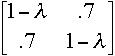
Consider the folllowing correlation matrix:
matrix list r

symmetric r[2,2]
    c1  c2
r1   1
r2  .7   1

matrix symeigen a l = r

/* eigenvalues */
matrix list l

l[1,2]
     e1   e2
r1  1.7   .3

matrix list a

/* eigenvectors */
symmetric a[2,2]
            e1          e2
r1   .70710678   .70710678
r2   .70710678  -.70710678
The equation for the eigenvalues can be expressed as solving for the determinant of
and setting it to zero, which reduces to
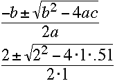
yields the two roots of 1.7 and .3. These roots are the eigenvalues also know as the characteristic values or characteristic roots. Once you have obtained the eigenvalues you use them to obtain a solution for the eigenvectors.
It is possible to interpret the eigenvectors directly but most researchers also look at the correlations between the components and the variables. These correlations are known as the component loadings.
Principal Components Analysis Example
The following example uses data for five socio-economic variables for 12 different locations. The variables are total population, median schooling, total employed, misc. professional services, and median housing value. The data are from Harman (1976).
use http://www.gseis.ucla.edu/courses/data/harman1
pca pop medsch employ profser medhouse, means
(obs=12)
Variable | Mean Std. Dev. Min Max
----------+----------------------------------------------------
pop | 6241.667 3439.994 1000 9900
medsch | 11.44167 1.786545 8.3 13.7
employ | 2333.333 1241.212 400 4000
profser | 120.8333 114.9275 10 390
medhouse | 17000 6367.531 9000 25000
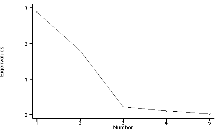
(principal components; 5 components retained)
Component Eigenvalue Difference Proportion Cumulative
------------------------------------------------------------------
1 2.87331 1.07665 0.5747 0.5747
2 1.79666 1.58182 0.3593 0.9340
3 0.21484 0.11490 0.0430 0.9770
4 0.09993 0.08468 0.0200 0.9969
5 0.01526 . 0.0031 1.0000
Eigenvectors
Variable | 1 2 3 4 5
----------+------------------------------------------------------
pop | 0.34273 0.60163 0.05952 0.20403 0.68950
medsch | 0.45251 -0.40641 0.68882 -0.35357 0.17486
employ | 0.39669 0.54167 0.24796 0.02294 -0.69801
profser | 0.55006 -0.07782 -0.66408 -0.50039 -0.00012
medhouse | 0.46674 -0.41643 -0.13965 0.76318 -0.08243
greigen
Next we will use data from the high school and beyond survey.
use http://www.gseis.ucla.edu/courses/data/hsb2

pca read write math science
(obs=200)

            (principal components; 4 components retained)
Component    Eigenvalue     Difference    Proportion    Cumulative
------------------------------------------------------------------
     1        2.85491         2.41937      0.7137         0.7137
     2        0.43554         0.06172      0.1089         0.8226
     3        0.37382         0.03810      0.0935         0.9161
     4        0.33573               .      0.0839         1.0000

               Eigenvectors
    Variable |      1          2          3          4
-------------+-------------------------------------------
        read |   0.50714   -0.22100   -0.54927    0.62632
       write |   0.48572    0.82012    0.27120    0.13393
        math |   0.51124   -0.05078   -0.38296   -0.76772
     science |   0.49550   -0.52535    0.69145    0.01980

pca read write math science, cov
(obs=200)

            (principal components; 4 components retained)
Component    Eigenvalue     Difference    Proportion    Cumulative
------------------------------------------------------------------
     1      272.11643       231.66023      0.7147         0.7147
     2       40.45620         3.10970      0.1063         0.8209
     3       37.34649         6.50385      0.0981         0.9190
     4       30.84264               .      0.0810         1.0000

               Eigenvectors
    Variable |      1          2          3          4
-------------+-------------------------------------------
        read |   0.54030   -0.19508   -0.73149   -0.36734
       write |   0.46626    0.79436    0.27230   -0.27829
        math |   0.48540    0.05035   -0.09084    0.86810
     science |   0.50504   -0.57306    0.61848   -0.18444

predict cs1 cs2
            (based on unrotated principal components)
            (2 scorings not used)

               Scoring Coefficients
    Variable |      1          2
-------------+---------------------
        read |   0.54030   -0.19508
       write |   0.46626    0.79436
        math |   0.48540    0.05035
     science |   0.50504   -0.57306

corr cs1 cs2
(obs=200)

             |      cs1      cs2
-------------+------------------
         cs1 |   1.0000
         cs2 |   0.0000   1.0000

regress socst read write math science

      Source |       SS       df       MS              Number of obs =     200
-------------+------------------------------           F(  4,   195) =   44.49
       Model |  10944.2858     4  2736.07144           Prob > F      =  0.0000
    Residual |  11991.9092   195  61.4969704           R-squared     =  0.4772
-------------+------------------------------           Adj R-squared =  0.4664
       Total |   22936.195   199  115.257261           Root MSE      =   7.842

------------------------------------------------------------------------------
       socst |      Coef.   Std. Err.      t    P>|t|     [95% Conf. Interval]
-------------+----------------------------------------------------------------
        read |    .380752   .0800116     4.76   0.000     .2229529    .5385511
       write |   .3751806   .0803521     4.67   0.000     .2167099    .5336512
        math |   .1322237   .0889155     1.49   0.139    -.0431359    .3075833
     science |  -.0279416   .0793993    -0.35   0.725    -.1845333      .12865
       _cons |   7.206027   3.611316     2.00   0.047     .0837748    14.32828
------------------------------------------------------------------------------

/* regression using  principal component scores */
regress socst cs1 cs2

      Source |       SS       df       MS              Number of obs =     200
-------------+------------------------------           F(  2,   197) =   83.68
       Model |  10535.0947     2  5267.54734           Prob > F      =  0.0000
    Residual |  12401.1003   197  62.9497478           R-squared     =  0.4593
-------------+------------------------------           Adj R-squared =  0.4538
       Total |   22936.195   199  115.257261           Root MSE      =  7.9341

------------------------------------------------------------------------------
       socst |      Coef.   Std. Err.      t    P>|t|     [95% Conf. Interval]
-------------+----------------------------------------------------------------
         cs1 |   .4307223   .0340952    12.63   0.000     .3634839    .4979607
         cs2 |   .2464224   .0884256     2.79   0.006     .0720402    .4208047
       _cons |   6.214682   3.632656     1.71   0.089    -.9492029    13.37857
------------------------------------------------------------------------------

/* anova using principal component scores */
anova cs1 prog

                           Number of obs =     200     R-squared     =  0.2154
                           Root MSE      = 14.6861     Adj R-squared =  0.2074

                  Source |  Partial SS    df       MS           F     Prob > F
              -----------+----------------------------------------------------
                   Model |  11661.6631     2  5830.83154      27.03     0.0000
                         |
                    prog |  11661.6631     2  5830.83154      27.03     0.0000
                         |
                Residual |  42489.5075   197  215.682779
              -----------+----------------------------------------------------
                   Total |  54151.1706   199  272.116435
Multivariate Course Page
Phil Ender, 15oct05, 25may02; 29jan98