Exploratory Factor Analysis

Multivariate Analysis

Exploratory Factor Analysis

Factor Analysis Model

Z = FA' [1]

That is,

z_j = a_j1F₁ + a_j2F₂ +...+ a_jpF_p

where

Z -> (nxm) standard score matrix
A -> (mxp) factor pattern matrix
F -> (nxp) factor score matrix

Factor Pattern

The factor pattern matrix, A, is the matrix of coefficients which applied to the factor scores reproduces the standard score matrix.

Factor Structure

S = Z'F/n = A(F'F/n) [2]

S -> (mxp) factor structure matrix

The factor structure matrix, S, is the matrix of correlations between factors and variables. Sometimes called the loading matrix. With orthogonal solutions the structure matrix and pattern matrix are the same.

Factor Correlations

Φ = F'F/n [3]

Φ -> (pxp) factor correlation matrix

If the factor analysis solution is orthogonal then Φ = I.

Fun with Math

Substituting into [2]

S = Z'F/n = A(F'F/n) [2]

we get

S = Z'F/n = A(F'F/n) = AΦ [4]

thus, when Φ = I, S = AI or S = A.

Reproduced Correlations

A = SΦ^-1

Since R = Z'Z/n [5]

R_r = AF'FA'/n = A(F'F/n)A' = AΦA'

R_r -> (mxm) matrix of reproduced correlations

Or equivalently, R_r = SA'

Variance to be Factored

Total variance       = h_j² + b_j² + e_j²
Reliability          = h_j² + b_j²
Communality      h_j² = h_j²
Uniqueness       d_j² =       b_j² + e_j²
Specificity      b_j² =       b_j²
Error            e_j² =             e_j²

PCA vs FA

Principal Components Analysis analyzes the total variance. That is, it analyzes the correlation matrix with one's in the diagonal.

Factor Analysis analyzes the common variance. Analyzes the correlation matrix with communality estimates in the diagonal. Sometimes called common factor analysis.

The Concept of Simple Structure

Each row in the factor pattern matrix should contain at least one zero.

Each column of the factor pattern matrix should contain at least m zeros.

Every pair of columns should contain rows whose loadings are zero in one column but non-zero in the other.

Every pair of columns should contain a large rows whose loadings are zero in both columns.

Every pair of columns should have only a few non-zero loadings in both columns.

Simple Structure Example

            Initial          Rotated
           Solution          Solution
          I  II III         F1  F2  F3
var1      X  X   0           0   0   X
var2      X  X   0           0   0   X
var3      X  X   0           0   0   X
var4      X -X   0           0   X   0
var5      X -X   0           0   X   0
var6      X  0   X           X   0   0
var7      X  0  -X           X   0   0
var8      X  0  -X           X   0   0
          G  B   B           P   P   P

Decisions in Factor Analysis

Method of initial factor solution
Method communality estimation
Number of factors to retain
Method of rotation

Method of Initial Factor Solution

Principal Axis Factor Analysis
Iterated Principal Axis Factor Analysis*
Image Factor Analysis
Alpha Factor Analysis
Maximum Likelihood Factor Analysis*
Unweighted Least Squares Factor Analysis
Generalized Least Squares Factor Analysis

Estimation of Communalities

SMC's*
Reliabilities
Largest off diagonal
Average Correlations
Centroid
Averoid

Number of Factors to Retain

Number of Eigenvalues greater than or equal to one (from the unreduced correlation matrix)
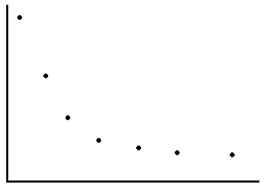
Scree Test/Scree Plot
Percent of variance
Hypothesis testing (ML)
Parallel analysis -- Monte Carlo (Humphreys & Ilgen, 1959; Montanelli & Humphreys, 1976)
Linn Method -- Monte Carlo (Linn, 1968)
Ender Method -- Quasi-Monte Carlo

Scree Plot

Methods of Rotation

Orthogonal Rotations

Varimax*
Varimax via the GPF algorithm*
Quartimax
Orthomax
Equamax
Parsimax
Minimum entropy
Comrey's tandem 1
Comrey's tandem 2

Oblique Rotations

Promax
Oblimin*
Oblimax
Quartimin
Biquartimin
Crawford-Ferguson*
Bentler's invariant pattern simplicity
Binormamin
Maxplane

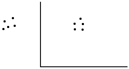
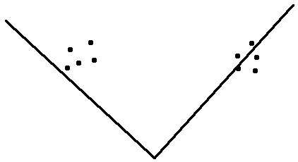
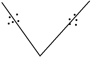
Rotating Example

Unrotated Factor Solution

Orthogonal Factor Solution

Oblique Factor Solution

The following example uses data for five socio-economic variables for 12 different locations. the variables are total population, median schooling, total employed, misc. professional services, and median housing value. The data are from Harman (1976).

Sample Size for Factor Analysis

There are a number of different guidelines given in the literature as to the appropriate sample size needed for factor analysis. I was taught that you needed at least 10 times as many observations as variables with a minimum of 200 observations. Pedhazur & Schmelkin (1991) suggest at least 50 observations per factor. Guadagnoli and Velicer (1988) have suggested a minimum sample size of 100 to 200 observations. Tabachnick & Fidell (1996) recommend at least 300 cases. And Comrey and Lee (1992) give the following guide for samples sizes: 50 as very poor, 100 as poor, 200 as fair, 300 as good, 500 as very good, and 1,000 as excellent.

Just remember, as with all statistical rules of thumb, your milage may vary.

Principal Axis Factor Analysis

use http://www.gseis.ucla.edu/courses/data/harman1, clear

factor pop medsch employ profser medhouse, pf fac(2)
(obs=12)

            (principal factors; 2 factors retained)
  Factor     Eigenvalue     Difference    Proportion    Cumulative
------------------------------------------------------------------
     1        2.73430         1.01823      0.6225         0.6225
     2        1.71607         1.67651      0.3907         1.0131
     3        0.03956         0.06409      0.0090         1.0221
     4       -0.02452         0.04808     -0.0056         1.0165
     5       -0.07261               .     -0.0165         1.0000

            Factor Loadings
 Variable |      1          2    Uniqueness
----------+--------------------------------
      pop |   0.62533    0.76621    0.02189
   medsch |   0.71370   -0.55515    0.18244
   employ |   0.71447    0.67936    0.02800
  profser |   0.87899   -0.15846    0.20226
 medhouse |   0.74215   -0.57806    0.11505

mat psi = e(Psi)'
mat com = J(rowsof(psi),1,1)
mat com = com - psi
mat colnames com=communalities
mat list com

com[5,1]
          communalities
     pop      .97811334
  medsch      .81756393
  employ      .97199928
 profser      .79774303
medhouse      .88495002

rotate, varimax normalize

Factor analysis/correlation                        Number of obs    =       12
    Method: principal factors                      Retained factors =        2
    Rotation: orthogonal varimax (Kaiser on)       Number of params =        9

    --------------------------------------------------------------------------
         Factor  |     Variance   Difference        Proportion   Cumulative
    -------------+------------------------------------------------------------
        Factor1  |      2.34986      0.24934            0.5349       0.5349
        Factor2  |      2.10051            .            0.4782       1.0131
    --------------------------------------------------------------------------
    LR test: independent vs. saturated:  chi2(10) =   60.63 Prob>chi2 = 0.0000

Rotated factor loadings (pattern matrix) and unique variances

    -------------------------------------------------
        Variable |  Factor1   Factor2 |   Uniqueness 
    -------------+--------------------+--------------
             pop |   0.0225    0.9887 |      0.0219  
          medsch |   0.9042    0.0006 |      0.1824  
          employ |   0.1462    0.9750 |      0.0280  
         profser |   0.7909    0.4151 |      0.2023  
        medhouse |   0.9407   -0.0000 |      0.1150  
    -------------------------------------------------

Factor rotation matrix

    --------------------------------
                 | Factor1  Factor2 
    -------------+------------------
         Factor1 |  0.7889   0.6145 
         Factor2 | -0.6145   0.7889 
    --------------------------------
    
rotate, oblique quartimin normalize 

Factor analysis/correlation                        Number of obs    =       12
    Method: principal factors                      Retained factors =        2
    Rotation: oblique quartimin (Kaiser on)        Number of params =        9

    --------------------------------------------------------------------------
         Factor  |     Variance   Proportion    Rotated factors are correlated
    -------------+------------------------------------------------------------
        Factor1  |      2.44531       0.5567
        Factor2  |      2.19402       0.4995
    --------------------------------------------------------------------------
    LR test: independent vs. saturated:  chi2(10) =   60.63 Prob>chi2 = 0.0000

Rotated factor loadings (pattern matrix) and unique variances

    -------------------------------------------------
        Variable |  Factor1   Factor2 |   Uniqueness 
    -------------+--------------------+--------------
             pop |  -0.0708    1.0001 |      0.0219  
          medsch |   0.9172   -0.0913 |      0.1824  
          employ |   0.0560    0.9736 |      0.0280  
         profser |   0.7630    0.3405 |      0.2023  
        medhouse |   0.9544   -0.0956 |      0.1150  
    -------------------------------------------------

Factor rotation matrix

    --------------------------------
                 | Factor1  Factor2 
    -------------+------------------
         Factor1 |  0.8463   0.6851 
         Factor2 | -0.5327   0.7284 
    --------------------------------


estat common

Correlation matrix of the Crawford-Ferguson(0) rotated common factors

    ----------------------------------
         Factors |  Factor1   Factor2 
    -------------+--------------------
         Factor1 |        1           
         Factor2 |    .1917         1 
    ----------------------------------

Remember, with oblique rotations you can get loadings greater than one.

Iterated Principal Axis Factor Analysis

factor pop medsch employ profser medhouse, ipf fac(2)
(obs=12)

Factor analysis/correlation                        Number of obs    =       12
    Method: iterated principal factors             Retained factors =        2
    Rotation: (unrotated)                          Number of params =        9

    Beware: solution is a Heywood case
            (i.e., invalid or boundary values of uniqueness)

    --------------------------------------------------------------------------
         Factor  |   Eigenvalue   Difference        Proportion   Cumulative
    -------------+------------------------------------------------------------
        Factor1  |      2.75653      1.01187            0.6124       0.6124
        Factor2  |      1.74466      1.71387            0.3876       1.0000
        Factor3  |      0.03079      0.03118            0.0068       1.0068
        Factor4  |     -0.00039      0.03002           -0.0001       1.0068
        Factor5  |     -0.03041            .           -0.0068       1.0000
    --------------------------------------------------------------------------
    LR test: independent vs. saturated:  chi2(10) =   60.63 Prob>chi2 = 0.0000

Factor loadings (pattern matrix) and unique variances

    -------------------------------------------------
        Variable |  Factor1   Factor2 |   Uniqueness 
    -------------+--------------------+--------------
             pop |   0.6300    0.7945 |     -0.0282  
          medsch |   0.7006   -0.5241 |      0.2344  
          employ |   0.6973    0.6710 |      0.0635  
         profser |   0.8808   -0.1470 |      0.2026  
        medhouse |   0.7789   -0.6057 |      0.0264  
    -------------------------------------------------

mat psi = e(Psi)'
mat com = J(rowsof(psi),1,1)
mat com = com - psi
mat colnames com=communalities
mat list com

com[5,1]
          communalities
     pop      1.0281865
  medsch      .76556374
  employ      .93651122
 profser       .7973836
medhouse      .97355023

rotate, varimax normalize

Factor analysis/correlation                        Number of obs    =       12
    Method: iterated principal factors             Retained factors =        2
    Rotation: orthogonal varimax (Kaiser on)       Number of params =        9

    Beware: solution is a Heywood case
            (i.e., invalid or boundary values of uniqueness)

    --------------------------------------------------------------------------
         Factor  |     Variance   Difference        Proportion   Cumulative
    -------------+------------------------------------------------------------
        Factor1  |      2.38417      0.26714            0.5297       0.5297
        Factor2  |      2.11703            .            0.4703       1.0000
    --------------------------------------------------------------------------
    LR test: independent vs. saturated:  chi2(10) =   60.63 Prob>chi2 = 0.0000

Rotated factor loadings (pattern matrix) and unique variances

    -------------------------------------------------
        Variable |  Factor1   Factor2 |   Uniqueness 
    -------------+--------------------+--------------
             pop |   0.0189    1.0138 |     -0.0282  
          medsch |   0.8749    0.0084 |      0.2344  
          employ |   0.1473    0.9565 |      0.0635  
         profser |   0.7894    0.4174 |      0.2026  
        medhouse |   0.9866   -0.0090 |      0.0264  
    -------------------------------------------------

Factor rotation matrix

    --------------------------------
                 | Factor1  Factor2 
    -------------+------------------
         Factor1 |  0.7950   0.6066 
         Factor2 | -0.6066   0.7950 
    --------------------------------

rotate, oblique quartimin normalize

Factor analysis/correlation                        Number of obs    =       12
    Method: iterated principal factors             Retained factors =        2
    Rotation: oblique quartimin (Kaiser on)        Number of params =        9

    Beware: solution is a Heywood case
            (i.e., invalid or boundary values of uniqueness)

    --------------------------------------------------------------------------
         Factor  |     Variance   Proportion    Rotated factors are correlated
    -------------+------------------------------------------------------------
        Factor1  |      2.47827       0.5506
        Factor2  |      2.20947       0.4909
    --------------------------------------------------------------------------
    LR test: independent vs. saturated:  chi2(10) =   60.63 Prob>chi2 = 0.0000

Rotated factor loadings (pattern matrix) and unique variances

    -------------------------------------------------
        Variable |  Factor1   Factor2 |   Uniqueness 
    -------------+--------------------+--------------
             pop |  -0.0767    1.0259 |     -0.0282  
          medsch |   0.8868   -0.0803 |      0.2344  
          employ |   0.0590    0.9547 |      0.0635  
         profser |   0.7614    0.3430 |      0.2026  
        medhouse |   1.0018   -0.1093 |      0.0264  
    -------------------------------------------------

Factor rotation matrix

    --------------------------------
                 | Factor1  Factor2 
    -------------+------------------
         Factor1 |  0.8515   0.6778 
         Factor2 | -0.5244   0.7353 
    --------------------------------

estat common

Correlation matrix of the quartimin rotated common factors

    ----------------------------------
         Factors |  Factor1   Factor2 
    -------------+--------------------
         Factor1 |        1           
         Factor2 |    .1915         1 
    ----------------------------------

Maximum Likelihood Factor Analysis

factor pop medsch employ profser medhouse, ml fac(2) (obs=12) Factor analysis/correlation Number of obs = 12 Method: maximum likelihood Retained factors = 2 Rotation: (unrotated) Number of params = 9 Schwarz's BIC = 26.0449 Log likelihood = -1.84039 (Akaike's) AIC = 21.6808 Beware: solution is a Heywood case (i.e., invalid or boundary values of uniqueness) -------------------------------------------------------------------------- Factor | Eigenvalue Difference Proportion Cumulative -------------+------------------------------------------------------------ Factor1 | 2.13887 -0.22952 0.4745 0.4745 Factor2 | 2.36839 . 0.5255 1.0000 -------------------------------------------------------------------------- LR test: independent vs. saturated: chi2(10) = 60.63 Prob>chi2 = 0.0000 LR test: 2 factors vs. saturated: chi2(1) = 2.50 Prob>chi2 = 0.1135 (tests formally not valid because a Heywood case was encountered) Factor loadings (pattern matrix) and unique variances ------------------------------------------------- Variable | Factor1 Factor2 | Uniqueness -------------+--------------------+-------------- pop | 1.0000 -0.0000 | 0.0000 medsch | 0.0098 0.9000 | 0.1900 employ | 0.9725 0.1179 | 0.0404 profser | 0.4389 0.7892 | 0.1844 medhouse | 0.0224 0.9600 | 0.0779 ------------------------------------------------- faform /* Available from ATS via the Internet */ Factor Loadings in Canonical Form 1 2 pop 0.62151 0.78340 medsch 0.71109 -0.55170 employ 0.69679 0.68853 profser 0.89106 -0.14672 medhouse 0.76602 -0.57911 mat psi = e(Psi)' mat com = J(rowsof(psi),1,1) mat com = com - psi mat colnames com=communalities mat list com com[5,1] communalities pop .99999969 medsch .81003767 employ .95956448 profser .81555395 medhouse .92206406 rotate, varimax normalize Factor analysis/correlation Number of obs = 12 Method: maximum likelihood Retained factors = 2 Rotation: orthogonal varimax (Kaiser on) Number of params = 9 Schwarz's BIC = 26.0449 Log likelihood = -1.84039 (Akaike's) AIC = 21.6808 Beware: solution is a Heywood case (i.e., invalid or boundary values of uniqueness) -------------------------------------------------------------------------- Factor | Variance Difference Proportion Cumulative -------------+------------------------------------------------------------ Factor1 | 2.38926 0.27125 0.5301 0.5301 Factor2 | 2.11801 . 0.4699 1.0000 -------------------------------------------------------------------------- LR test: independent vs. saturated: chi2(10) = 60.63 Prob>chi2 = 0.0000 LR test: 2 factors vs. saturated: chi2(1) = 2.50 Prob>chi2 = 0.1135 (tests formally not valid because a Heywood case was encountered) Rotated factor loadings (pattern matrix) and unique variances ------------------------------------------------- Variable | Factor1 Factor2 | Uniqueness -------------+--------------------+-------------- pop | 0.0213 0.9998 | 0.0000 medsch | 0.9000 -0.0095 | 0.1900 employ | 0.1387 0.9697 | 0.0404 profser | 0.7984 0.4219 | 0.1844 medhouse | 0.9603 0.0019 | 0.0779 ------------------------------------------------- Factor rotation matrix -------------------------------- | Factor1 Factor2 -------------+------------------ Factor1 | 0.0213 Factor2 | 0.9998 -0.0213 -------------------------------- rotate, oblique quartimin normalize Factor analysis/correlation Number of obs = 12 Method: maximum likelihood Retained factors = 2 Rotation: oblique quartimin (Kaiser on) Number of params = 9 Schwarz's BIC = 26.0449 Log likelihood = -1.84039 (Akaike's) AIC = 21.6808 Beware: solution is a Heywood case (i.e., invalid or boundary values of uniqueness) -------------------------------------------------------------------------- Factor | Variance Proportion Rotated factors are correlated -------------+------------------------------------------------------------ Factor1 | 2.48025 0.5503 Factor2 | 2.20740 0.4897 -------------------------------------------------------------------------- LR test: independent vs. saturated: chi2(10) = 60.63 Prob>chi2 = 0.0000 LR test: 2 factors vs. saturated: chi2(1) = 2.50 Prob>chi2 = 0.1135 (tests formally not valid because a Heywood case was encountered) Rotated factor loadings (pattern matrix) and unique variances ------------------------------------------------- Variable | Factor1 Factor2 | Uniqueness -------------+--------------------+-------------- pop | -0.0700 1.0106 | 0.0000 medsch | 0.9131 -0.0981 | 0.1900 employ | 0.0517 0.9687 | 0.0404 profser | 0.7706 0.3488 | 0.1844 medhouse | 0.9732 -0.0925 | 0.0779 ------------------------------------------------- Factor rotation matrix -------------------------------- | Factor1 Factor2 -------------+------------------ Factor1 | 0.1179 0.9976 Factor2 | 0.9930 0.0688 -------------------------------- estat common Correlation matrix of the quartimin rotated common factors ---------------------------------- Factors | Factor1 Factor2 -------------+-------------------- Factor1 | 1 Factor2 | .1859 1 ---------------------------------- How to Do It

Create reduced correlation matrix, R1, by replacing the diagonal elements of the correleation matrix with SMC's

SMC's are obtained as follows:

where each r^jj is a diagonal element of R^-1.

Now do the same as in Principal Components Analysis using R₁ instead of R.

Factor Scores

In common-factor analysis the scores on the common factors are estimated rather than determined from the scores on the observed variables.

It is mathematically impossible to determine uniquely or exactly the common-factor scores even if the population correlations are known.

This is know as factor indeterminacy.

Factor score estimation is done by a variation of the multiple regression procedure.

F = ZR_xx^-1AR_xx

where Z -> Standard scores
A -> Factor pattern matrix
R_zz -> Correlations among the variables R_xx -> Correlation among the factors

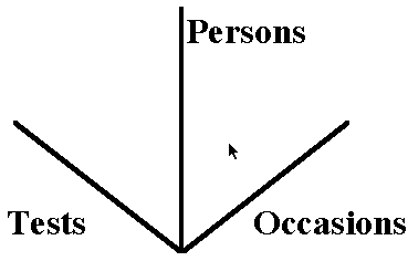
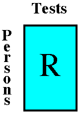
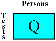
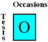
Types of Factor Analysis

R Factor Analysis

Q Factor Analysis

P Factor Analysis

O Factor Analysis

S Factor Analysis

T Factor Analysis

Stata Example

Here is an example using the api99g dataset.

use http://www.gseis.ucla.edu/courses/data/api99g, clear

keep if stype==1 /* use only elementary schools */
(1773 observations deleted)

summarize meals ell yr_rnd acs_k3 acs_46 avg_ed full enroll

    Variable |     Obs        Mean   Std. Dev.       Min        Max
-------------+-----------------------------------------------------
       meals |    4421    51.88102   31.07313          0        100
         ell |    4421    25.19204   22.91157          0         95
      yr_rnd |    4421    1.178919   .3833277          1          2
      acs_k3 |    4359    19.29571   1.539583         12         31
      acs_46 |    4294    28.90452    3.21889         14         50
      avg_ed |    4257    2.749298   .7542556          1          5
        full |    4420    87.86357   13.35186         13        100
      enroll |    4397    426.9616   175.8747        101       1570

univar meals ell yr_rnd acs_k3 acs_46 avg_ed full enroll

                                        -------------- Quantiles --------------
Variable       n     Mean     S.D.      Min      .25      Mdn      .75      Max
-------------------------------------------------------------------------------
   meals    4421    51.88    31.07     0.00    24.00    53.00    79.00   100.00
     ell    4421    25.19    22.91     0.00     6.00    18.00    40.00    95.00
  yr_rnd    4421     1.18     0.38     1.00     1.00     1.00     1.00     2.00
  acs_k3    4359    19.30     1.54    12.00    19.00    19.00    20.00    31.00
  acs_46    4294    28.90     3.22    14.00    27.00    29.00    31.00    50.00
  avg_ed    4257     2.75     0.75     1.00     2.17     2.71     3.26     5.00
    full    4420    87.86    13.35    13.00    81.00    92.00   100.00   100.00
  enroll    4397   426.96   175.87   101.00   303.00   403.00   523.00  1570.00
-------------------------------------------------------------------------------

corr meals ell yr_rnd acs_k3 acs_46 avg_ed full enroll
(obs=4059)

             |    meals      ell   yr_rnd   acs_k3   acs_46   avg_ed     full   enroll
-------------+------------------------------------------------------------------------
       meals |   1.0000
         ell |   0.7716   1.0000
      yr_rnd |   0.3027   0.3158   1.0000
      acs_k3 |  -0.0251   0.0275   0.0016   1.0000
      acs_46 |  -0.0274   0.0077   0.0522   0.2788   1.0000
      avg_ed |  -0.8392  -0.6818  -0.2842  -0.0193   0.0288   1.0000
        full |  -0.5145  -0.5146  -0.2592   0.0344  -0.0304   0.4036   1.0000
      enroll |   0.1984   0.3092   0.5125   0.1374   0.2017  -0.1645  -0.2696   1.0000

factor meals ell yr_rnd acs_k3 acs_46 avg_ed full enroll, ml
(obs=4059)
number of factors adjusted to 4

Factor analysis/correlation                        Number of obs    =     4059
    Method: maximum likelihood                     Retained factors =        4
    Rotation: (unrotated)                          Number of params =       26
                                                   Schwarz's BIC    =  225.553
    Log likelihood = -4.763415                     (Akaike's) AIC   =  61.5268

    Beware: solution is a Heywood case
            (i.e., invalid or boundary values of uniqueness)

    --------------------------------------------------------------------------
         Factor  |   Eigenvalue   Difference        Proportion   Cumulative
    -------------+------------------------------------------------------------
        Factor1  |      1.55692     -0.93102            0.2975       0.2975
        Factor2  |      2.48794      1.53599            0.4754       0.7728
        Factor3  |      0.95195      0.71491            0.1819       0.9547
        Factor4  |      0.23705            .            0.0453       1.0000
    --------------------------------------------------------------------------
    LR test: independent vs. saturated:  chi2(28) = 1.3e+04 Prob>chi2 = 0.0000
    LR test:   4 factors vs. saturated:  chi2(2)  =    9.51 Prob>chi2 = 0.0086
    (tests formally not valid because a Heywood case was encountered)

Factor loadings (pattern matrix) and unique variances

    ---------------------------------------------------------------------
        Variable |  Factor1   Factor2   Factor3   Factor4 |   Uniqueness 
    -------------+----------------------------------------+--------------
           meals |   0.1984    0.9058   -0.0057    0.1342 |      0.1222  
             ell |   0.3092    0.7430    0.0226    0.2775 |      0.2749  
          yr_rnd |   0.5125    0.2211   -0.0618    0.0030 |      0.6846  
          acs_k3 |   0.1374   -0.0538    0.9340    0.0133 |      0.1058  
          acs_46 |   0.2017   -0.0780    0.2640    0.0249 |      0.8829  
          avg_ed |  -0.1645   -0.9192   -0.0522    0.1914 |      0.0887  
            full |  -0.2696   -0.4612    0.0540   -0.3234 |      0.6070  
          enroll |   1.0000   -0.0000   -0.0000   -0.0000 |      0.0000  
    ---------------------------------------------------------------------

/*  don't display small loadings */

factor, blanks(.2)
(obs=4059)

Factor analysis/correlation                        Number of obs    =     4059
    Method: maximum likelihood                     Retained factors =        4
    Rotation: (unrotated)                          Number of params =       26
                                                   Schwarz's BIC    =  225.553
    Log likelihood = -4.763415                     (Akaike's) AIC   =  61.5268

    Beware: solution is a Heywood case
            (i.e., invalid or boundary values of uniqueness)

    --------------------------------------------------------------------------
         Factor  |   Eigenvalue   Difference        Proportion   Cumulative
    -------------+------------------------------------------------------------
        Factor1  |      1.55692     -0.93102            0.2975       0.2975
        Factor2  |      2.48794      1.53599            0.4754       0.7728
        Factor3  |      0.95195      0.71491            0.1819       0.9547
        Factor4  |      0.23705            .            0.0453       1.0000
    --------------------------------------------------------------------------
    LR test: independent vs. saturated:  chi2(28) = 1.3e+04 Prob>chi2 = 0.0000
    LR test:   4 factors vs. saturated:  chi2(2)  =    9.51 Prob>chi2 = 0.0086
    (tests formally not valid because a Heywood case was encountered)

Factor loadings (pattern matrix) and unique variances

    ---------------------------------------------------------------------
        Variable |  Factor1   Factor2   Factor3   Factor4 |   Uniqueness 
    -------------+----------------------------------------+--------------
           meals |             0.9058                     |      0.1222  
             ell |   0.3092    0.7430              0.2775 |      0.2749  
          yr_rnd |   0.5125    0.2211                     |      0.6846  
          acs_k3 |                       0.9340           |      0.1058  
          acs_46 |   0.2017              0.2640           |      0.8829  
          avg_ed |            -0.9192                     |      0.0887  
            full |  -0.2696   -0.4612             -0.3234 |      0.6070  
          enroll |   1.0000                               |      0.0000  
    ---------------------------------------------------------------------
    (blanks represent abs(loading)<.2)

/* parallel analysis for eigenvalues 
   compare the eigenvalues of the factor analysis 
   with eigenvalues of randomly generated variables 
   to assist in determing the number of factors. 
*/

fapara, seed(123456789)   /* Available from ATS via the Internet */
(obs=4421)

Parallel Analysis for Eigenvalues

      Eigen   Random      Dif
c1   2.8288   0.0646   2.7642
c2   0.7448   0.0407   0.7041
c3   0.3042   0.0257   0.2785
c4   0.0692   0.0202   0.0490
c5  -0.0720  -0.0167  -0.0553
c6  -0.1129  -0.0338  -0.0792
c7  -0.1929  -0.0417  -0.1512
c8  -0.2339  -0.0468  -0.1870

quietly factor meals ell yr_rnd acs_k3 acs_46 avg_ed full enroll, ml fact(3)

rotate, oblique quartimin normalize blanks(.2)


Factor analysis/correlation                        Number of obs    =     4059
    Method: maximum likelihood                     Retained factors =        3
    Rotation: oblique quartimin (Kaiser on)        Number of params =       21
                                                   Schwarz's BIC    =  334.796
    Log likelihood = -80.15692                     (Akaike's) AIC   =  202.314

    Beware: solution is a Heywood case
            (i.e., invalid or boundary values of uniqueness)

    --------------------------------------------------------------------------
         Factor  |     Variance   Proportion    Rotated factors are correlated
    -------------+------------------------------------------------------------
        Factor1  |      2.81012       0.5623
        Factor2  |      1.56721       0.3136
        Factor3  |      1.14509       0.2291
    --------------------------------------------------------------------------
    LR test: independent vs. saturated:  chi2(28) = 1.3e+04 Prob>chi2 = 0.0000
    LR test:   3 factors vs. saturated:  chi2(7)  =  160.10 Prob>chi2 = 0.0000
    (tests formally not valid because a Heywood case was encountered)

Rotated factor loadings (pattern matrix) and unique variances

    -----------------------------------------------------------
        Variable |  Factor1   Factor2   Factor3 |   Uniqueness 
    -------------+------------------------------+--------------
           meals |   0.9941                     |      0.0530  
             ell |   0.7733                     |      0.3411  
          yr_rnd |             0.5045           |      0.6591  
          acs_k3 |                       1.0281 |      0.0000  
          acs_46 |                       0.2684 |      0.8883  
          avg_ed |  -0.8898                     |      0.2570  
            full |  -0.4828                     |      0.6853  
          enroll |             0.9353           |      0.1186  
    -----------------------------------------------------------
    (blanks represent abs(loading)<.2)

Factor rotation matrix

    -----------------------------------------
                 | Factor1  Factor2  Factor3 
    -------------+---------------------------
         Factor1 | -0.0156   0.0850   0.9877 
         Factor2 |  0.9977   0.3905  -0.0347 
         Factor3 | -0.0664   0.9167   0.1523 
    -----------------------------------------

predict f1 f2 f3
(regression scoring assumed)

Scoring coefficients (method = regression; based on quartimin rotated factors)

    --------------------------------------------
        Variable |  Factor1   Factor2   Factor3 
    -------------+------------------------------
           meals |  0.75089   0.00327  -0.07235 
             ell |  0.09436   0.05264  -0.00078 
          yr_rnd |  0.01758   0.08515   0.01184 
          acs_k3 | -0.00759  -0.04124   0.96686 
          acs_46 | -0.00164   0.02344   0.00389 
          avg_ed | -0.13741   0.00746   0.01452 
            full | -0.03079  -0.03137  -0.00200 
          enroll |  0.05156   0.86936   0.13329 
    --------------------------------------------

corr f1 f2 f3
(obs=4059)

             |       f1       f2       f3
-------------+---------------------------
          f1 |   1.0000
          f2 |   0.3453   1.0000
          f3 |  -0.0588   0.2052   1.0000

The three factors can be interpreted as follows. Factor 1 seems to reflect socioeconomic variables. Factor 2 appears to be related to the size of the population in the school neighborhoods, while Factor 3 is concerned with classroom size.

Stata 9 & above allows for the following methods for initial factor extraction:

      pf      principal-axis factor analysis; the default
      pcf     principal-components factor analysis
      ipf     iterated principal-axis factor analysis
      ml      maximum-likelihood factor analysis

The following options are allowed with the factor command:

      factors(#)     maximum number of factors to be retained
      mineigen(#)    minimum value of eigenvalues to be retained
      citerate(#)    communality re-estimation iterations (ipf only)

The factor commands has the following post-estimation procedures:

      estat anti           anti-image correlation and covariance matrices
      estat common         correlation matrix of the common factors
      estat factors        AIC and BIC model selection criteria for different numbers of
                             factors
      estat kmo            Kaiser-Meyer-Olkin measure of sampling adequacy
      estat residuals      matrix of correlation residuals
      estat rotatecompare  compare rotated and unrotated loadings
      estat smc            squared multiple correlations between each variable and the rest
      estat structure      correlations between variables and common factors
      estat summarize      estimation sample summary
      loadingplot          plot factor loadings
      rotate               rotate factor loadings
      scoreplot            plot score variables
      screeplot            plot eigenvalues

The following factor rotation procedures are available in Stata 9 using the rotate command:

      varimax          varimax (orthogonal only); the default
      vgpf             varimax via the GPF algorithm (orthogonal only)
      quartimax        quartimax (orthogonal only)
      equamax          equamax (orthogonal only)
      parsimax         parsimax (orthogonal only)
      entropy          minimum entropy (orthogonal only)
      tandem1          Comrey's tandem 1 principle (orthogonal only)
      tandem2          Comrey's tandem 2 principle (orthogonal only)

      promax[(#)]      promax power # (implies oblique); default is promax(3)
      oblimin[(#)]     oblimin with gamma=#; default is oblimin(0)
      cf(#)            Crawford-Ferguson family with kappa=#, 0<=#<1
      bentler          Bentler's invariant pattern simplicity
      oblimax          oblimax
      quartimin        quartimin
      target(Tg)       rotate towards matrix Tg
      partial(Tg W)    rotate towards matrix Tg, weighted by matrix W

The rotate command has the following options:

      orthogonal         restrict to orthogonal rotations; default, except with promax()
      oblique            allow oblique rotations
      rotation_methods   rotation criterion
      normalize          rotate Horst normalized matrix
      horst              synonym for normalize
      factors(#)         rotate # factors or components; default all
      components(#)      synonym for factors()

Multivariate Course Page

Phil Ender, 16nov05, 15oct05, 29Jan98