According to Webster
In the beginning...
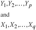
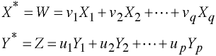
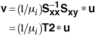
Consider two sets of variables:
Construct
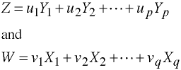
Construct the linear combinations:
Such that rzw is a maximum.
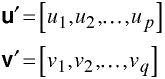
Let
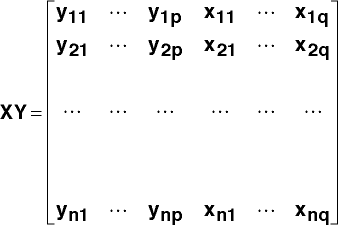
The XY Matrix
Consider a matrix XY made up of p Y's and q X's.
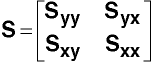
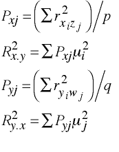
Partitioning the Covariance Matrix
Let S be the XY covariance matrix, thus,
And
Thus, the sum of squared deviation scores can be obtained without transforming the raw scores.
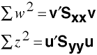
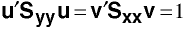
Criteria
Choose u and v such that
Compute
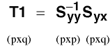
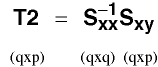
Now let
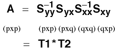
Let μi2 = eigenvalues of A
Let u = eigenvectors of A
Next let
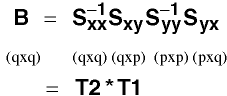
A & B will have the same eigenvalues.
Let v = eigenvectors of B.
Computing v
Let
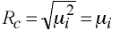
Canonical Correlation
Eigenvalues of A are canonical correlations squared, therefore
Computational Notes
Matrix A is not symmetric so we will need to go through some additional steps in order to get the eigenvalues and eigenvectors using the symeigen command.
1)  C = Syx*Sxx-1*Sxy
2)  F = cholesky(Syy-1)
3)  D = F'*C*F
4)  symeigen W L = D    /* L has eigenvalues  of A */
5)  U = F*W             /* U has eigenvectors of A */
Remember the elements of L are μi2
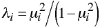
Different Eigenvalues
Each canonical correlation has an eigenvalue related to Wilks' Lambda.
Tests of Significance
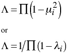
Wilks' Lambdas
Compute m = n -3/2 - (p+q)/2 once.
The following are repeated with one being subtracted from p and q until either is equal to one. Thus,
First time     p=3    q=5
Second time    p=2    q=4
Third time     p=1    q=3
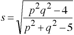
df1 = pq
df2 = ms - pq/2 + 1
Rao's F Approximation
with df1 and df2 degrees of freedom.
Canonical Redundancy Coefficients
A measure of association between two sets of variables.
This measure is asymmetric:
R2x.y is the redundancy of set X given set Y
R2y.x is the redundancy of set Y given set X.
Canonical Redundancy Note
Rc2 is an estimate of the shared variance of two linear combinations of variables and not of the variance of the variables themselves. Thus, even when Rc2 is high, the redundancy of Y, X, or both may be very low.
Although it is always possible to compute both R2x.y and R2y.x, it is not always the case that both redundancy measures are meaningful. For example, when the Y variables are true dependent variables, R2y.x is useful while R2x.y does not make sense.
Redundancy
Each is a weighted sum of the squared canonical correlations, proportional to the aggregate variance of the variables in the set accounted for by successive canonical variates of that set.
What Canonical Correlation Analysis Does...
Best
Questions concerning the number and nature of mutually independent relations (dimensions) between two sets of variables.
Mediocre
Questions concerning the degree of overlap or redundancy between two sets of variables.
Not Very Well
Questions concerning the similarity between two within-set correlation or covariance matrices.
Stata Example
Stata has completely rewritten their canonical correlation procedure in Stata 9.
use http://www.philender.com/courses/data/timm, clear

canon (apt ppvt rpmt) (n s ns na ss), test(1 2 3)


Linear combinations for canonical correlations         Number of obs =      37
------------------------------------------------------------------------------
             |      Coef.   Std. Err.      t    P>|t|     [95% Conf. Interval]
-------------+----------------------------------------------------------------
u1           |
         apt |   .0032264   .0082904     0.39   0.699    -.0135873      .02004
        ppvt |   .0762248   .0152914     4.98   0.000     .0452124    .1072372
        rpmt |   .0141323   .0588196     0.24   0.811    -.1051594    .1334239
-------------+----------------------------------------------------------------
v1           |
           n |  -.0071509    .082705    -0.09   0.932    -.1748843    .1605826
           s |  -.0756585   .0465969    -1.62   0.113    -.1701612    .0188443
          ns |  -.0353218   .0450604    -0.78   0.438    -.1267084    .0560649
          na |   .1579155    .051318     3.08   0.004     .0538377    .2619933
          ss |   .0435563   .0544885     0.80   0.429    -.0669515     .154064
-------------+----------------------------------------------------------------
u2           |
         apt |   -.033176   .0151245    -2.19   0.035      -.06385    -.002502
        ppvt |  -.0016715   .0278969    -0.06   0.953     -.058249     .054906
        rpmt |   .2756473   .1073075     2.57   0.014     .0580176     .493277
-------------+----------------------------------------------------------------
v2           |
           n |   .1599911   .1508828     1.06   0.296    -.1460134    .4659955
           s |    .042124   .0850089     0.50   0.623    -.1302821    .2145302
          ns |   .2381605   .0822059     2.90   0.006     .0714393    .4048817
          na |  -.0594188    .093622    -0.63   0.530    -.2492931    .1304555
          ss |  -.1823911    .099406    -1.83   0.075    -.3839959    .0192137
-------------+----------------------------------------------------------------
u3           |
         apt |   .0358057    .030764     1.16   0.252    -.0265865    .0981979
        ppvt |  -.0482553   .0567435    -0.85   0.401    -.1633363    .0668258
        rpmt |   .2104353   .2182681     0.96   0.341     -.232233    .6531035
-------------+----------------------------------------------------------------
v3           |
           n |   .0992871   .3069021     0.32   0.748    -.5231393    .7217135
           s |   .1746239   .1729119     1.01   0.319    -.1760577    .5253054
          ns |  -.0100806   .1672103    -0.06   0.952    -.3491988    .3290376
          na |  -.2290303   .1904313    -1.20   0.237    -.6152428    .1571822
          ss |   .2019493   .2021962     1.00   0.325    -.2081236    .6120222
------------------------------------------------------------------------------
                                     (Standard errors estimated conditionally)
Canonical correlations:
  0.7165  0.4906  0.2668

----------------------------------------------------------------------------
Tests of significance of all canonical correlations

                         Statistic      df1      df2            F     Prob>F
         Wilks' lambda     .343169       15  80.4576       2.5381     0.0039 a
        Pillai's trace     .825289       15       93       2.3529     0.0066 a
Lawley-Hotelling trace     1.44876       15       83       2.6722     0.0023 a
    Roy's largest root     1.05512        5       31       6.5417     0.0003 u
----------------------------------------------------------------------------
Test of significance of canonical correlations 1-3

                         Statistic      df1      df2            F     Prob>F
         Wilks' lambda     .343169       15  80.4576       2.5381     0.0039 a
----------------------------------------------------------------------------
Test of significance of canonical correlations 2-3

                         Statistic      df1      df2            F     Prob>F
         Wilks' lambda     .705252        8       60       1.4308     0.2025 e
----------------------------------------------------------------------------
Test of significance of canonical correlation 3

                         Statistic      df1      df2            F     Prob>F
         Wilks' lambda      .92883        3       31       0.7918     0.5078 e
----------------------------------------------------------------------------
                            e = exact, a = approximate, u = upper bound on F

canon, stdcoef


Canonical correlation analysis                         Number of obs =      37

Standardized coefficients for the first variable set

                 |        1         2         3
    -------------+------------------------------
             apt |   0.0713   -0.7332    0.7913
            ppvt |   0.9548   -0.0209   -0.6044
            rpmt |   0.0437    0.8531    0.6513
    --------------------------------------------


Standardized coefficients for the second variable set

                 |        1         2         3
    -------------+------------------------------
               n |  -0.0211    0.4719    0.2928
               s |  -0.3835    0.2135    0.8850
              ns |  -0.2244    1.5132   -0.0640
              na |   1.1438   -0.4304   -1.6589
              ss |   0.2774   -1.1618    1.2864
    --------------------------------------------

Canonical correlations:
  0.7165  0.4906  0.2668

estat correlations

Correlations for variable list 1

                 |      apt      ppvt      rpmt
    -------------+------------------------------
             apt |   1.0000
            ppvt |   0.3703    1.0000
            rpmt |   0.2114    0.3548    1.0000
    --------------------------------------------

Correlations for variable list 2

                 |        n         s        ns        na        ss
    -------------+--------------------------------------------------
               n |   1.0000
               s |   0.4007    1.0000
              ns |   0.5370    0.3523    1.0000
              na |   0.6481    0.6478    0.7136    1.0000
              ss |   0.6704    0.4252    0.7695    0.7951    1.0000
    ----------------------------------------------------------------

Correlations between variable lists 1 and 2

                 |      apt      ppvt      rpmt
    -------------+------------------------------
               n |   0.1860    0.4444    0.3504
               s |   0.1609    0.2682    0.2386
              ns |   0.0685    0.4692    0.4388
              na |   0.2617    0.6720    0.3390
              ss |   0.3341    0.5876    0.3404
    --------------------------------------------


estat loadings

Canonical loadings for variable list 1

                 |        1         2         3
    -------------+------------------------------
             apt |   0.4341   -0.5606    0.7052
            ppvt |   0.9967    0.0102   -0.0803
            rpmt |   0.3976    0.6906    0.6041
    --------------------------------------------

Canonical loadings for variable list 2

                 |        1         2         3
    -------------+------------------------------
               n |   0.6320    0.3122    0.4004
               s |   0.3879    0.1630    0.4521
              ns |   0.6588    0.6406    0.2112
              na |   0.9422    0.1697    0.0814
              ss |   0.8371    0.0675    0.4906
    --------------------------------------------

Correlation between variable list 1 and canonical variates from list 2

                 |        1         2         3
    -------------+------------------------------
             apt |   0.3111   -0.2750    0.1881
            ppvt |   0.7142    0.0050   -0.0214
            rpmt |   0.2849    0.3388    0.1612
    --------------------------------------------

Correlation between variable list 2 and canonical variates from list 1

                 |        1         2         3
    -------------+------------------------------
               n |   0.4529    0.1532    0.1068
               s |   0.2780    0.0800    0.1206
              ns |   0.4721    0.3143    0.0563
              na |   0.6751    0.0833    0.0217
              ss |   0.5998    0.0331    0.1309
    --------------------------------------------

canred 1  /* findit canred */

Canonical redundancy analysis for canonical correlation 1

Canonical correlation coefficient          0.7165
Squared canonical correlation coefficient  0.5134

                                       own    opposite
Proportion of standardized variance  variate   variate
           of u variables with ...    0.4467    0.2293
           of v variables with ...    0.5145    0.2641

canred 2  /* findit canred */

Canonical redundancy analysis for canonical correlation 2

Canonical correlation coefficient          0.4906
Squared canonical correlation coefficient  0.2407

                                       own    opposite
Proportion of standardized variance  variate   variate
           of u variables with ...    0.2638    0.0635
           of v variables with ...    0.1136    0.0273
Multivariate Course Page
Phil Ender, 2may05, 29Jan98