Multivariate Analysis
Discriminant Analysis
Discriminant analysis, also known as linear discriminant function analysis,
combines aspects of multivariate analysis of varicance
with the ability to classify observations into known categories. It is a useful adjunct in
helping to interpret the results of manova. It provides an alternative to multinomial
logistic regression that will function adequately with somewhat smaller sample sizes. Like
so many multivariate techniques it does require that the dependent variables come
from a multivariate normal distribution.
What does discriminant analysis do?
Tests multivariate differences between groups -- really the same as manova
Determines the dimensionality of the group differences
Provides information on the relative importance or contribution of each variable
Classifies known and unknown observations into groups
In the beginning...
Let Y be a linear combination of p dependent variables, such that
Total deviation SSCP
Let T be the Total deviation SSCP matrix, which is obtained from
Within Groups deviation SSCP
The within group sums of squares and cross products matrix is expressed as:
Between Groups deviation SSCP
where
which has n1 rows of means from group 1, n2 rows of means from groups 2,
nk rows of means from group k, and where
However, it is easier to obtain B by taking T - W.
The between groups sums of squares for the linear combination is:

Discriminant Analysis
We wish to select the elements of v such that  is
a maximum.
is
a maximum.
This occurs when (B - λW)v = 0. Thus, discriminant analysis reduces
to finding the eigenvalues and eigenvectors of W-1B which is often written E-1H.
Computational Note
W-1B is generally non-symmetric. Most matrix languages cannot compute the eigenvalues
and vectors unless the matrix is symmetric. Therefore, you must perform some additional
computations to obtain the eigenvalues and eigenvectors.
mat l = cholesky(W)          /* Cholesky decomposition */
mat u = l'                   /* u equals l transpose   */
mat a = inv(l)*B*inv(u)      /* a is symmetric */
mat symeigen uv e = a        /* e will have the eigenvalues of W-1B */
mat v = inv(u)*uv            /* v will have the eigenvectors of W-1B */
Aside
The cholesky function performs the Cholesky decomposition of a matrix such that if
L = cholesky(A) then L'L = A, where L is lower triangular matrix. The formula could also be be
written LU = A where U is upper triangular. Matrix A must be symmetric and nonnegative definite.
Number of Dimensions
The maximum number of discriminant dimensions is Min(p, k-1).
Trimming
Trim the eigenvalues and eigenvectors
Retain only as many as the number of eigenvalues greater than zero.
Let E be the trimmed matrix of eigenvalues.
Let V be the trimmed matrix of eigenvectors.
Standardized Discriminant Weights
Standardized discriminant weights or coefficients are used when all the variables are in standard score from.
Standardized discriminant coefficients are one of the pieces used in the interpretation of the
discriminant analysis.
wii is a diagonal matrix whose elements are the square roots of the diagonal elements of W.
Then let 
sv is the vector of standardized discriminant coefficients.
Structure Matrix
The structure matrix gives the correlations between the variables and the discriminant functions.
The structure matrix is another of the pieces used in the interpretation of the discriminant analysis.
Computing the structure matrix.
mat E = V'*W*V
mat F = inv(sqrt(diag(E)))
mat G = inv(sqet(diag(W)))
mat A = G*W*V*F
A is the structure matrix.
Canonical Correlations
Wilks' Lambda
Using Canonical Correlations
Let t = 1 - Rc2
then,
2-Group Case
Discuss the 2-group case.
>Chi-square
with degrees of freedom:
let q = k-1
For Chisquare1 = pq
For Chisquare2 = (p-1)*(q-1)
For Chisquare3 = (p-2)*(q-2)
2-Group Example
There are new discriminant analyse procedures in Stata 10. We will be using
the candisc or discrim lda command for these examples. candisc is
a wrapper program for discrim lad which includes a number of commonly used
options.
use http://www.philender.com/courses/data/honors, clear
describe
Contains data from http://www.gseis.ucla.edu/courses/data/honors.dta
obs: 200
vars: 7 14 Dec 2001 09:19
size: 6,400 (99.9% of memory free)
-------------------------------------------------------------------------------
storage display value
variable name type format label variable label
-------------------------------------------------------------------------------
id float %9.0g
female float %9.0g fl
ses float %9.0g sl
lang float %9.0g language test score
math float %9.0g math score
science float %9.0g science score
honors float %9.0g
candisc female lang, group(honors)
Canonical linear discriminant analysis
| | Like-
| Canon. Eigen- Variance | lihood
Fcn | Corr. value Prop. Cumul. | Ratio F df1 df2 Prob>F
----+---------------------------------+------------------------------------
1 | 0.5166 .364005 1.0000 1.0000 | 0.7331 35.854 2 197 0.0000 e
---------------------------------------------------------------------------
Ho: this and smaller canon. corr. are zero; e = exact F
Standardized canonical discriminant function coefficients
| function1
-------------+-----------
female | .3706778
lang | .9822288
Canonical structure
| function1
-------------+-----------
female | .2328554
lang | .9302168
Group means on canonical variables
honors | function1
-------------+-----------
0 | -.3604546
1 | .9997513
Resubstitution classification summary
+---------+
| Key |
|---------|
| Number |
| Percent |
+---------+
| Classified
True honors | 0 1 | Total
-------------+----------------+-------
0 | 114 33 | 147
| 77.55 22.45 | 100.00
| |
1 | 16 37 | 53
| 30.19 69.81 | 100.00
-------------+----------------+-------
Total | 130 70 | 200
| 65.00 35.00 | 100.00
| |
Priors | 0.5000 0.5000 |
/* display raw discriminant coefficients */
matrix list e(L_unstd)
e(L_unstd)[3,1]
function1
female .74791853
lang .10957945
_cons -6.1309503
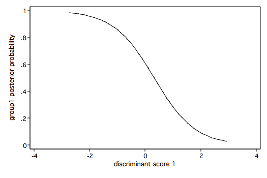
predict pr, pr
predict dsc, dsc
twoway line pr dsc, sort
3-Group Example
use http://www.philender.com/courses/data/hsb2, clear
(highschool and beyond (200 cases))
/* equivalent to one-way anova */
candisc write, group(prog) notable nostruct
Canonical linear discriminant analysis
| | Like-
| Canon. Eigen- Variance | lihood
Fcn | Corr. value Prop. Cumul. | Ratio F df1 df2 Prob>F
----+---------------------------------+------------------------------------
1 | 0.4215 .215987 1.0000 1.0000 | 0.8224 21.275 2 197 0.0000 e
---------------------------------------------------------------------------
Ho: this and smaller canon. corr. are zero; e = exact F
Standardized canonical discriminant function coefficients
| function1
-------------+-----------
write | 1
Group means on canonical variables
prog | function1
-------------+-----------
general | -.1668754
academic | .4030641
vocation | -.6962467
/* compare with */
anova write prog
Number of obs = 200 R-squared = 0.1776
Root MSE = 8.63918 Adj R-squared = 0.1693
Source | Partial SS df MS F Prob > F
-----------+----------------------------------------------------
Model | 3175.69786 2 1587.84893 21.27 0.0000
|
prog | 3175.69786 2 1587.84893 21.27 0.0000
|
Residual | 14703.1771 197 74.635417
-----------+----------------------------------------------------
Total | 17878.875 199 89.843593
display sqrt(e(r2))
.42145333
/* equivalent to one-way manova */
candisc write read math, group(prog) nostruct
Canonical linear discriminant analysis
| | Like-
| Canon. Eigen- Variance | lihood
Fcn | Corr. value Prop. Cumul. | Ratio F df1 df2 Prob>F
----+---------------------------------+------------------------------------
1 | 0.5125 .356283 0.9874 0.9874 | 0.7340 10.87 6 390 0.0000 e
2 | 0.0672 .004543 0.0126 1.0000 | 0.9955 .44518 2 196 0.6414 e
---------------------------------------------------------------------------
Ho: this and smaller canon. corr. are zero; e = exact F
Standardized canonical discriminant function coefficients
| function1 function2
-------------+----------------------
write | .3310784 1.183414
read | .2728524 -.4097932
math | .5815538 -.655658
Group means on canonical variables
prog | function1 function2
-------------+----------------------
general | -.3120021 .1190423
academic | .5358515 -.0196809
vocation | -.8444861 -.0658081
Resubstitution classification summary
+---------+
| Key |
|---------|
| Number |
| Percent |
+---------+
| Classified
True prog | general academic vocation | Total
-------------+------------------------------+---------
general | 11 17 17 | 45
| 24.44 37.78 37.78 | 100.00
| |
academic | 18 68 19 | 105
| 17.14 64.76 18.10 | 100.00
| |
vocation | 14 7 29 | 50
| 28.00 14.00 58.00 | 100.00
-------------+------------------------------+---------
Total | 43 92 65 | 200
| 21.50 46.00 32.50 | 100.00
| |
Priors | 0.3333 0.3333 0.3333 |
/* display manova table */
estat manova
Number of obs = 200
W = Wilks' lambda L = Lawley-Hotelling trace
P = Pillai's trace R = Roy's largest root
Source | Statistic df F(df1, df2) = F Prob>F
-----------+--------------------------------------------------
prog | W 0.7340 2 6.0 390.0 10.87 0.0000 e
| P 0.2672 6.0 392.0 10.08 0.0000 a
| L 0.3608 6.0 388.0 11.67 0.0000 a
| R 0.3563 3.0 196.0 23.28 0.0000 u
|--------------------------------------------------
Residual | 197
-----------+--------------------------------------------------
Total | 199
--------------------------------------------------------------
e = exact, a = approximate, u = upper bound on F
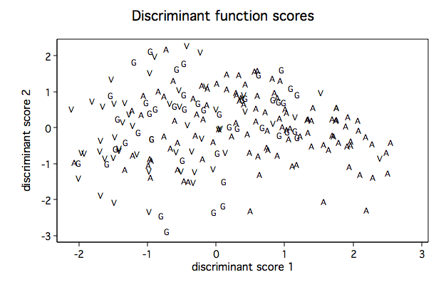
label define sel 1 "G" 2 "A" 3 "V", modify
scoreplot, msymbol(i)
 /* compare discriminant analysis with manova */
manova write read math = prog
Number of obs = 200
W = Wilks' lambda L = Lawley-Hotelling trace
P = Pillai's trace R = Roy's largest root
Source | Statistic df F(df1, df2) = F Prob>F
-----------+--------------------------------------------------
prog | W 0.7340 2 6.0 390.0 10.87 0.0000 e
| P 0.2672 6.0 392.0 10.08 0.0000 a
| L 0.3608 6.0 388.0 11.67 0.0000 a
| R 0.3563 3.0 196.0 23.28 0.0000 u
|--------------------------------------------------
Residual | 197
-----------+--------------------------------------------------
Total | 199
--------------------------------------------------------------
e = exact, a = approximate, u = upper bound on F
/* compare discriminant analysis with manova */
manova write read math = prog
Number of obs = 200
W = Wilks' lambda L = Lawley-Hotelling trace
P = Pillai's trace R = Roy's largest root
Source | Statistic df F(df1, df2) = F Prob>F
-----------+--------------------------------------------------
prog | W 0.7340 2 6.0 390.0 10.87 0.0000 e
| P 0.2672 6.0 392.0 10.08 0.0000 a
| L 0.3608 6.0 388.0 11.67 0.0000 a
| R 0.3563 3.0 196.0 23.28 0.0000 u
|--------------------------------------------------
Residual | 197
-----------+--------------------------------------------------
Total | 199
--------------------------------------------------------------
e = exact, a = approximate, u = upper bound on F
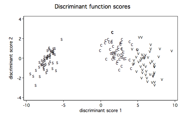
Fisher's Iris Data
This example makes use of the classic Iris data that R. A. Fisher used in developing the
linear discriminant function.
use http://www.philender.com/courses/data/iris, clear

describe

Contains data from http://www.gseis.ucla.edu/courses/data/iris.dta
  obs:           150
 vars:             6                          17 Feb 2000 14:30
 size:         4,200 (99.9% of memory free)
-------------------------------------------------------------------------------
              storage  display     value
variable name   type   format      label      variable label
-------------------------------------------------------------------------------
case            float  %9.0g
type            float  %10.0g      tl         type of iris
sl              float  %9.0g                  sepal length
sw              float  %9.0g                  sepal width
pl              float  %9.0g                  petal length
pw              float  %9.0g                  petal width
-------------------------------------------------------------------------------
Sorted by:  type

tabulate type

    type of |
       iris |      Freq.     Percent        Cum.
------------+-----------------------------------
     setosa |         50       33.33       33.33
 versicolor |         50       33.33       66.67
  virginica |         50       33.33      100.00
------------+-----------------------------------
      Total |        150      100.00


candisc sl sw pl pw, group(type)

Canonical linear discriminant analysis

      |                                 | Like-
      | Canon.   Eigen-     Variance    | lihood
  Fcn | Corr.    value   Prop.   Cumul. | Ratio     F      df1    df2  Prob>F
  ----+---------------------------------+------------------------------------
    1 | 0.9848  32.1919  0.9912  0.9912 | 0.0234  199.15     8    288  0.0000 e
    2 | 0.4712  .285391  0.0088  1.0000 | 0.7780  13.794     3    145  0.0000 e
  ---------------------------------------------------------------------------
  Ho: this and smaller canon. corr. are zero;                     e = exact F

Standardized canonical discriminant function coefficients

                 | function1  function2
    -------------+----------------------
              sl | -.4269549  -.0124077
              sw | -.5212416  -.7352612
              pl |  .9472573   .4010379
              pw |  .5751607  -.5810398

Canonical structure

                 | function1  function2
    -------------+----------------------
              sl |  .2225959  -.3108118
              sw | -.1190115  -.8636809
              pl |  .7060654  -.1677014
              pw |  .6331779  -.7372421

Group means on canonical variables

            type | function1  function2
    -------------+----------------------
          setosa |   -7.6076   -.215133
      versicolor |  1.825049   .7278996
       virginica |   5.78255  -.5127666

Resubstitution classification summary

    +---------+
    | Key     |
    |---------|
    | Number  |
    | Percent |
    +---------+
                 | Classified
    True type    |     setosa  versicolor   virginica |      Total
    -------------+------------------------------------+-----------
          setosa |         50           0           0 |         50
                 |     100.00        0.00        0.00 |     100.00
                 |                                    |
      versicolor |          0          48           2 |         50
                 |       0.00       96.00        4.00 |     100.00
                 |                                    |
       virginica |          0           1          49 |         50
                 |       0.00        2.00       98.00 |     100.00
    -------------+------------------------------------+-----------
           Total |         50          49          51 |        150
                 |      33.33       32.67       34.00 |     100.00
                 |                                    |
          Priors |     0.3333      0.3333      0.3333 |

estat manova

                           Number of obs =     150

                           W = Wilks' lambda      L = Lawley-Hotelling trace
                           P = Pillai's trace     R = Roy's largest root

                  Source |  Statistic     df   F(df1,    df2) =   F   Prob>F
              -----------+--------------------------------------------------
                    type | W   0.0234      2     8.0   288.0   199.15 0.0000 e
                         | P   1.1919            8.0   290.0    53.47 0.0000 a
                         | L  32.4773            8.0   286.0   580.53 0.0000 a
                         | R  32.1919            4.0   145.0  1166.96 0.0000 u
                         |--------------------------------------------------
                Residual |               147
              -----------+--------------------------------------------------
                   Total |               149
              --------------------------------------------------------------
                           e = exact, a = approximate, u = upper bound on F

label define tl 1 "S" 2 "C" 3 "V", modify

scoreplot, msymbol(i)
One More Example
use http://www.philender.com/courses/data/hsb2

egen grp = group(prog female)

/* findit tablist */

tablist grp prog female, sort(v) nol clean

    grp   prog   female   Freq
      1      1        0     21
      2      1        1     24
      3      2        0     47
      4      2        1     58
      5      3        0     23
      6      3        1     27

candisc read write math science socst, group(grp)

Canonical linear discriminant analysis

      |                                 | Like-
      | Canon.   Eigen-     Variance    | lihood
  Fcn | Corr.    value   Prop.   Cumul. | Ratio     F      df1    df2  Prob>F
  ----+---------------------------------+------------------------------------
    1 | 0.5782  .502254  0.6132  0.6132 | 0.4975  5.8498    25  707.3  0.0000 a
    2 | 0.4363   .23516  0.2871  0.9003 | 0.7474  3.6511    16  584.2  0.0000 a
    3 | 0.2197  .050705  0.0619  0.9622 | 0.9231  1.7353     9  467.4  0.0786 a
    4 | 0.1728  .030785  0.0376  0.9997 | 0.9699  1.4843     4    386  0.2062 e
    5 | 0.0144  .000207  0.0003  1.0000 | 0.9998  .04025     1    194  0.8412 e
  ---------------------------------------------------------------------------
  Ho: this and smaller canon. corr. are zero;  e = exact F, a = approximate F

Standardized canonical discriminant function coefficients

                 | function1  function2  function3  function4  function5
    -------------+-------------------------------------------------------
            read | -.1161169  -.4829687   .1886365   1.321818   .1538771
           write | -.6602812   1.128027   -.212974   .1360569   .4061492
            math |  -.463602  -.5339929   .8257989  -.7658781   .3940945
         science |  .6107802  -.3927407  -1.125132  -.3845829   .2800101
           socst | -.3563766   -.225085  -.2689487  -.3519051  -1.088045

Canonical structure

                 | function1  function2  function3  function4  function5
    -------------+-------------------------------------------------------
            read | -.5809872  -.5235904  -.2656326   .5296293   .1929744
           write | -.8095514   .2094842   -.443327   .0312908   .3212865
            math | -.6837577  -.5135297   .0156334  -.2991848   .4230919
         science | -.2778489  -.4341668  -.7449201  -.1238876   .4050248
           socst | -.7035231  -.2935881  -.3890976  -.0536654  -.5143777

Group means on canonical variables

             grp | function1  function2  function3  function4  function5
    -------------+-------------------------------------------------------
               1 |  .6640051  -.4587528  -.4351828   .2093051  -.0166562
               2 |  .1637273   .6219646  -.1688396  -.3557218  -.0124101
               3 | -.3608076  -.4947248  -.0729075  -.1062484   .0169581
               4 | -.7733276   .0895048   .1406045   .0935383  -.0099369
               5 |  1.315385  -.3706178   .4039811  -.0541723  -.0050263
               6 |   .506798   .7885798  -.0307032   .1835678    .020094

Resubstitution classification summary

    +---------+
    | Key     |
    |---------|
    | Number  |
    | Percent |
    +---------+
                 | Classified
    True grp     |      1       2       3       4       5       6 |  Total
    -------------+------------------------------------------------+-------
               1 |      5       2       3       1       7       3 |     21
                 |  23.81    9.52   14.29    4.76   33.33   14.29 | 100.00
                 |                                                |
               2 |      0      10       1       5       4       4 |     24
                 |   0.00   41.67    4.17   20.83   16.67   16.67 | 100.00
                 |                                                |
               3 |      5       6      17      13       3       3 |     47
                 |  10.64   12.77   36.17   27.66    6.38    6.38 | 100.00
                 |                                                |
               4 |      1       9      11      25       4       8 |     58
                 |   1.72   15.52   18.97   43.10    6.90   13.79 | 100.00
                 |                                                |
               5 |      5       4       1       1      12       0 |     23
                 |  21.74   17.39    4.35    4.35   52.17    0.00 | 100.00
                 |                                                |
               6 |      3       4       2       2       4      12 |     27
                 |  11.11   14.81    7.41    7.41   14.81   44.44 | 100.00
    -------------+------------------------------------------------+-------
           Total |     19      35      35      47      34      30 |    200
                 |   9.50   17.50   17.50   23.50   17.00   15.00 | 100.00
                 |                                                |
          Priors | 0.1667  0.1667  0.1667  0.1667  0.1667  0.1667 |

estat manova

                           Number of obs =     200

                           W = Wilks' lambda      L = Lawley-Hotelling trace
                           P = Pillai's trace     R = Roy's largest root

                  Source |  Statistic     df   F(df1,    df2) =   F   Prob>F
              -----------+--------------------------------------------------
                     grp | W   0.4975      5    25.0   707.3     5.85 0.0000 a
                         | P   0.6031           25.0   970.0     5.32 0.0000 a
                         | L   0.8191           25.0   942.0     6.17 0.0000 a
                         | R   0.5023            5.0   194.0    19.49 0.0000 u
                         |--------------------------------------------------
                Residual |               194
              -----------+--------------------------------------------------
                   Total |               199
              --------------------------------------------------------------
                           e = exact, a = approximate, u = upper bound on F
Multivariate Course Page
Phil Ender, 13jul07, 28oct05, 23apr05, 29Jan98