Multilevel Data Issues

Linear Statistical Models: Regression

Multilevel Data Issues

Updated for Stata 11

What is Appropriate Unit of Analysis?

The individual student?

the class?

the school?

the school district?

the state?

Comments & Opinions

Sherif, 1963 - Even within a given discipline, researchers use different units of analysis depending, among other things, on the theoretical orientation and the type of variables and measures they use.

Hannan & Young, 1976 - "Despite the long history of concern and the recent upsurge of interest in the problem, a great deal of current research practice appears virtually unaffected."

Cronbach, 1976 - "The majority of studies of educational effects - whether classroom experiments, or evaluations of programs, or surveys - have collected and analyzed data in ways that have concealed more than they reveal. The established methods have generated false conclusions in many studies."

Cross-level inferences

When findings obtained from data collected using one unit of analysis are used to make inferences about another unit of analysis.

Example: correlations between IQ & achievement made at the school level used to draw conclusions about correlations among individual students.

Most discussions of cross-level inference are concerned with inferences made from aggregates to individuals.

A Question?

Why not study the relation between variables using the unit of interest?

It may not be feasible to collect data on individuals or to match data for individuals across variables.

Some Examples

(Thorndike, 1939) - Correlation bewteen IQ and number of pupils per room for 12 districts. Within each district r = 0. When districts were aggregated into one large group, r = .45. When the averages for IQ and room size were used, r = .90

(Robinson, 1950) - Correlation between race and literacy, in individuals r = .203. When aggregated at the state level, r = .773.

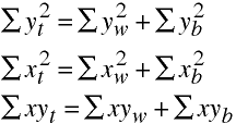
Three Partitions

Within Groups
Between Groups
Total

Partitioning Sums of Squares

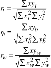
Correlations

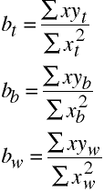
Regression Coefficients

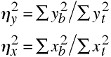
Eta Squared

Eta squared is equal to R² when doing regression using coded vectors for group membership.

Correlations Again

Using eta squared the formulas for the correlations can be rewritten as:

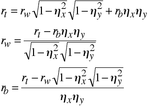
Regression Coefficients Again

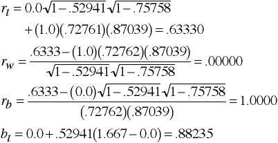
An Example

Source Σy² Σx² Σxy r b
Total 82.5 42.5 37.5 .633 .88235
G1 10.0 10.0 0 0 0
G2 10.0 10.0 0 0 0
Within 20.0 20.0 0 0 0
Between 62.5 22.5 37.5 1.00 1.667

Source	Σy²	Σx²	Σxy	r	b
Total	82.5	42.5	37.5	.633	.88235
G1	10.0	10.0	0	0	0
G2	10.0	10.0	0	0	0
Within	20.0	20.0	0	0	0
Between	62.5	22.5	37.5	1.00	1.667

eta²_y = .75758
eta²_x = .52941

Multilevel Analysis

Some argue that the issue is not appropriate unit of analysis but development of appropriate techniques that will make full use of information from different levels.

The choice of one level to the exclusion of others may result in masking certain effects or in indicating effects when none exist.

Multilevel analyses are most important when individuals are nested within groups and groups are nested within larger units.

Say, students nested in classes and classes nested in schools.

Some processes work on individuals while others work on groups.

(Cronbach & Webb, 1975) - High mean aptitude of a class may lead a teacher to crowd more material into the course, thereby leading to either greater or lesser achievement for the class as a whole.

"...the experience of a student with an IQ of 110 depends on whether the class mean is 100 or 120."

Multilevel data analysis is currently one of the hottest research areas.

The program HLM (Hierarchical Linear Models) is the most commonly used multilevel data analysis in the US. HLM was developed by Bryk and Radenbush.

Really cutting edge work is being done with multilevel analysis of latent variables (structural equation models).

Stata Example

The sch10 dataset contains data on students in 10 schools.

use http://www.philender.com/courses/data/sch10, clear

rename scid school

table school, cont(freq mean math mean hmwk) format(%6.2f)

----------------------------------------------
group(sch |
id)       |      Freq.  mean(math)  mean(hmwk)
----------+-----------------------------------
        1 |         23       45.74        1.39
        2 |         20       42.15        2.35
        3 |         24       53.25        1.83
        4 |         22       43.55        1.64
        5 |         22       49.86        0.86
        6 |         20       46.40        1.15
        7 |         67       62.82        3.30
        8 |         21       49.67        2.10
        9 |         21       46.33        1.33
       10 |         20       47.85        1.60
----------------------------------------------

regress math

      Source |       SS       df       MS              Number of obs =     260
-------------+------------------------------           F(  0,   259) =    0.00
       Model |        0.00     0           .           Prob > F      =       .
    Residual |    32116.60   259  124.002317           R-squared     =  0.0000
-------------+------------------------------           Adj R-squared =  0.0000
       Total |    32116.60   259  124.002317           Root MSE      =  11.136

------------------------------------------------------------------------------
        math |      Coef.   Std. Err.      t    P>|t|     [95% Conf. Interval]
-------------+----------------------------------------------------------------
       _cons |       51.3   .6906026    74.28   0.000     49.94009    52.65991
------------------------------------------------------------------------------

regress math hmwk

      Source |       SS       df       MS              Number of obs =     260
-------------+------------------------------           F(  1,   258) =   84.64
       Model |  7933.80702     1  7933.80702           Prob > F      =  0.0000
    Residual |   24182.793   258  93.7317557           R-squared     =  0.2470
-------------+------------------------------           Adj R-squared =  0.2441
       Total |    32116.60   259  124.002317           Root MSE      =  9.6815

------------------------------------------------------------------------------
        math |      Coef.   Std. Err.      t    P>|t|     [95% Conf. Interval]
-------------+----------------------------------------------------------------
        hmwk |   3.571856   .3882366     9.20   0.000      2.80734    4.336372
       _cons |   44.07386    .988641    44.58   0.000     42.12703    46.02069
------------------------------------------------------------------------------

sort school

by school: generate i = _n

egen mmath = mean(math), by(school)

egen mhmwk = mean(hmwk), by(school)

regress mmath if i==1 [aw=n]
(sum of wgt is   2.6000e+02)

      Source |       SS       df       MS              Number of obs =      10
-------------+------------------------------           F(  0,     9) =    0.00
       Model |        0.00     0           .           Prob > F      =       .
    Residual |  539.635975     9  59.9595528           R-squared     =  0.0000
-------------+------------------------------           Adj R-squared =  0.0000
       Total |  539.635975     9  59.9595528           Root MSE      =  7.7434

------------------------------------------------------------------------------
       mmath |      Coef.   Std. Err.      t    P>|t|     [95% Conf. Interval]
-------------+----------------------------------------------------------------
       _cons |       51.3   2.448664    20.95   0.000     45.76074    56.83926
------------------------------------------------------------------------------

regress mmath mhmwk if i==1 [aw=n]
(sum of wgt is   2.6000e+02)

      Source |       SS       df       MS              Number of obs =      10
-------------+------------------------------           F(  1,     8) =   14.33
       Model |  346.267285     1  346.267285           Prob > F      =  0.0054
    Residual |   193.36869     8  24.1710863           R-squared     =  0.6417
-------------+------------------------------           Adj R-squared =  0.5969
       Total |  539.635975     9  59.9595528           Root MSE      =  4.9164

------------------------------------------------------------------------------
       mmath |      Coef.   Std. Err.      t    P>|t|     [95% Conf. Interval]
-------------+----------------------------------------------------------------
       mhmwk |   7.014745   1.853336     3.78   0.005     2.740944    11.28855
       _cons |   37.10863   4.058993     9.14   0.000     27.74858    46.46869
------------------------------------------------------------------------------

regress math hmwk mhmwk

      Source |       SS       df       MS              Number of obs =     260
-------------+------------------------------           F(  2,   257) =   67.00
       Model |  11006.6159     2  5503.30794           Prob > F      =  0.0000
    Residual |  21109.9841   257  82.1400161           R-squared     =  0.3427
-------------+------------------------------           Adj R-squared =  0.3376
       Total |    32116.60   259  124.002317           Root MSE      =  9.0631

------------------------------------------------------------------------------
        math |      Coef.   Std. Err.      t    P>|t|     [95% Conf. Interval]
-------------+----------------------------------------------------------------
        hmwk |   2.136635   .4326083     4.94   0.000     1.284726    2.988543
       mhmwk |    4.87811    .797556     6.12   0.000     3.307533    6.448687
       _cons |   37.10863   1.467442    25.29   0.000     34.21889    39.99837
------------------------------------------------------------------------------

statsby "regress math hmwk" _b[_cons] _b[hmwk] , by(school) clear

command:     regress math hmwk
by:          school
statistics:  _stat1 = _b[_cons]
             _stat2 = _b[hmwk]

list

        school     _stat1     _stat2
  1.         1   50.68354  -3.553797
  2.         2   49.01229  -2.920123
  3.         3      38.75   7.909091
  4.         4   34.39382   5.592664
  5.         5   53.93863  -4.718411
  6.         6   49.25896  -2.486056
  7.         7   59.21022    1.09464
  8.         8   36.05535    6.49631
  9.         9      38.52       5.86
 10.        10   37.71392   6.335052

use http://www.philender.com/courses/data/sch10, clear

xtmixed math hmwk || school: hnwk, var cov(unstr)

Performing EM optimization: 

Performing gradient-based optimization: 

Iteration 0:   log restricted-likelihood = -881.97717  
Iteration 1:   log restricted-likelihood = -881.97717  

Computing standard errors:

Mixed-effects REML regression                   Number of obs      =       260
Group variable: school                          Number of groups   =        10

                                                Obs per group: min =        20
                                                               avg =      26.0
                                                               max =        67


                                                Wald chi2(1)       =      1.72
Log restricted-likelihood = -881.97717          Prob > chi2        =    0.1892

------------------------------------------------------------------------------
        math |      Coef.   Std. Err.      z    P>|z|     [95% Conf. Interval]
-------------+----------------------------------------------------------------
        hmwk |   2.040464   1.554221     1.31   0.189    -1.005754    5.086682
       _cons |   44.77059   2.743654    16.32   0.000     39.39313    50.14806
------------------------------------------------------------------------------

------------------------------------------------------------------------------
  Random-effects Parameters  |   Estimate   Std. Err.     [95% Conf. Interval]
-----------------------------+------------------------------------------------
school: Unstructured         |
                   var(hmwk) |   22.45281   11.50929      8.221395     61.3191
                  var(_cons) |   69.30461    35.0263       25.7376    186.6192
             cov(hmwk,_cons) |  -31.76199   18.17669     -67.38764    3.863666
-----------------------------+------------------------------------------------
               var(Residual) |   43.07098   3.929865      36.01802    51.50505
------------------------------------------------------------------------------
LR test vs. linear regression:       chi2(3) =   151.64   Prob > chi2 = 0.0000

/* rerun to get hmwk, _cons correlation */

xtmixed

Mixed-effects REML regression                   Number of obs      =       260
Group variable: school                          Number of groups   =        10

                                                Obs per group: min =        20
                                                               avg =      26.0
                                                               max =        67


                                                Wald chi2(1)       =      1.72
Log restricted-likelihood = -881.97717          Prob > chi2        =    0.1892

------------------------------------------------------------------------------
        math |      Coef.   Std. Err.      z    P>|z|     [95% Conf. Interval]
-------------+----------------------------------------------------------------
        hmwk |   2.040464   1.554221     1.31   0.189    -1.005754    5.086682
       _cons |   44.77059   2.743654    16.32   0.000     39.39313    50.14806
------------------------------------------------------------------------------

------------------------------------------------------------------------------
  Random-effects Parameters  |   Estimate   Std. Err.     [95% Conf. Interval]
-----------------------------+------------------------------------------------
school: Unstructured         |
                    sd(hmwk) |   4.738439    1.21446      2.867297    7.830652
                   sd(_cons) |   8.324939   2.103697      5.073224    13.66086
            corr(hmwk,_cons) |  -.8051768   .1242568     -.9473872   -.3975028
-----------------------------+------------------------------------------------
                sd(Residual) |   6.562849   .2994024      6.001501    7.176702
------------------------------------------------------------------------------
LR test vs. linear regression:       chi2(3) =   151.64   Prob > chi2 = 0.0000

Note: LR test is conservative and provided only for reference.

Linear Statistical Models Course

Phil Ender, 17sep10, 29Jan98