Polynomial regression can be used to fit a regression line to a curved set of points. Contrary to how it sounds, curvilinear regression uses a linear model to fit a curved line to data points. Curvilinear regression makes use of various transformations of variables to achieve its fit. An example of a curvilinear model is
Curvilinear regression should not be confused with nonlinear regression (NL). Nonlinear regression fits arbitrary nonlinear functions to the dependent variable. An example of a nonlinear model is
Example 1
From Pedhazur (1997), a study looks at practice time (x) in minutes and the number of correct responses (y).
Stata Curvilinear Regression Program
use http://www.philender.com/courses/data/curve, clear

scatter y x
Remarks
From Pedhazur (1997), a study looks at practice time (x) in minutes and the number of correct responses (y). Inspection of the y vs x plot reveals a degree of curvilinearity.
Based upon the scatterplot we will try three models:
model 1 -- y = bo + b1x + e -- linear
model 2 -- y = bo + b1x + b2x2 + e -- quadratic
model 3 -- y = bo + b1x + b2x2 +
b3x3 + e -- cubic
regress y x   /* linear */

  Source |       SS       df       MS                  Number of obs =      18
---------+------------------------------               F(  1,    16) =   32.72
   Model |  380.112798     1  380.112798               Prob > F      =  0.0000
Residual |  185.887202    16  11.6179501               R-squared     =  0.6716
---------+------------------------------               Adj R-squared =  0.6511
   Total |      566.00    17  33.2941176               Root MSE      =  3.4085

------------------------------------------------------------------------------
       y |      Coef.   Std. Err.       t     P>|t|       [95% Conf. Interval]
---------+--------------------------------------------------------------------
       x |   1.284165   .2245067      5.720   0.000       .8082319    1.760098
   _cons |    4.89154    1.73176      2.825   0.012       1.220372    8.562708
------------------------------------------------------------------------------

regress y c.x##c.x   /* linear and quadratic */

      Source |       SS       df       MS              Number of obs =      18
-------------+------------------------------           F(  2,    15) =   31.90
       Model |  458.245766     2  229.122883           Prob > F      =  0.0000
    Residual |  107.754234    15  7.18361562           R-squared     =  0.8096
-------------+------------------------------           Adj R-squared =  0.7842
       Total |         566    17  33.2941176           Root MSE      =  2.6802

------------------------------------------------------------------------------
           y |      Coef.   Std. Err.      t    P>|t|     [95% Conf. Interval]
-------------+----------------------------------------------------------------
           x |   4.151667   .8872181     4.68   0.000     2.260607    6.042728
             |
     c.x#c.x |   -.209529   .0635329    -3.30   0.005    -.3449462   -.0741119
             |
       _cons |  -2.236083    2.55445    -0.88   0.395    -7.680764    3.208598
------------------------------------------------------------------------------

regress y c.x##c.x##c.x   /* linear, quadratic and cubic */

      Source |       SS       df       MS              Number of obs =      18
-------------+------------------------------           F(  3,    14) =   20.30
       Model |  460.224174     3  153.408058           Prob > F      =  0.0000
    Residual |  105.775826    14  7.55541616           R-squared     =  0.8131
-------------+------------------------------           Adj R-squared =  0.7731
       Total |         566    17  33.2941176           Root MSE      =  2.7487

------------------------------------------------------------------------------
           y |      Coef.   Std. Err.      t    P>|t|     [95% Conf. Interval]
-------------+----------------------------------------------------------------
           x |   2.267499   3.792818     0.60   0.559    -5.867288    10.40229
             |
     c.x#c.x |   .0975798   .6036817     0.16   0.874    -1.197189    1.392348
             |
 c.x#c.x#c.x |  -.0144026   .0281457    -0.51   0.617    -.0747692     .045964
             |
       _cons |   .7460164     6.3894     0.12   0.909    -12.95788    14.44992
------------------------------------------------------------------------------

test x c.x#c.x

 ( 1)  x = 0
 ( 2)  c.x#c.x = 0

       F(  2,    14) =   15.21
            Prob > F =    0.0003

/* rerun regression with linear and quadratic */

regress y c.x##c.x

[output omitted]

predict p

scatter y p x, msym(o i) con(. l)
Remarks
From the above analysis, it appears that model 2 appears to be our best bet.
The linear model is
y = -2.236083 + 4.151667x -0.209529x2. A plot of y vs x with
the predicted scores connect by a curved line is displayed above.
Example 2
Here is another artifical example. This time we are looking at the relationship between test perfromance and anxiety.
input anxiety perform
1  11
1  13
2  24
2  20
3  42
3  36
4  48
4  42
5  46
5  38
6  23
6  19
7   9
7  11
end
These data graph into an inverted-U shape. Let's run a second degree polynomial regression.
scatter perform anxietyregress perform c.anxiety##c.anxiety Source | SS df MS Number of obs = 14 -------------+------------------------------ F( 2, 11) = 44.51 Model | 2334.38095 2 1167.19048 Prob > F = 0.0000 Residual | 288.47619 11 26.2251082 R-squared = 0.8900 -------------+------------------------------ Adj R-squared = 0.8700 Total | 2622.85714 13 201.758242 Root MSE = 5.121 ------------------------------------------------------------------------------ perform | Coef. Std. Err. t P>|t| [95% Conf. Interval] -------------+---------------------------------------------------------------- anxiety | 29.63095 3.23401 9.16 0.000 22.51294 36.74896 | c.anxiety#| c.anxiety | -3.72619 .3950972 -9.43 0.000 -4.595794 -2.856587 | _cons | -16.71429 5.643117 -2.96 0.013 -29.1347 -4.293868 ------------------------------------------------------------------------------ predict p scatter perform p anxiety, msym(o i) con(. l)
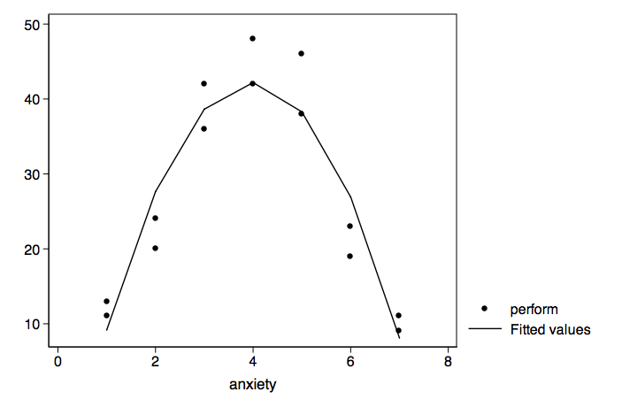
In social psychology, this inverted-U curve is called the Yerkes-Dodson curve.
Example 3
Let's try this using the hsb2 dataset.
use http://www.philender.com/courses/data/hsbdemo, clear scatter math write, jitter(2)regress math write Source | SS df MS Number of obs = 200 -------------+------------------------------ F( 1, 198) = 122.00 Model | 6658.72246 1 6658.72246 Prob > F = 0.0000 Residual | 10807.0725 198 54.5811744 R-squared = 0.3812 -------------+------------------------------ Adj R-squared = 0.3781 Total | 17465.795 199 87.7678141 Root MSE = 7.3879 ------------------------------------------------------------------------------ math | Coef. Std. Err. t P>|t| [95% Conf. Interval] -------------+---------------------------------------------------------------- write | .6102747 .0552524 11.05 0.000 .501316 .7192334 _cons | 20.43775 2.962373 6.90 0.000 14.5959 26.2796 ------------------------------------------------------------------------------ linktest Source | SS df MS Number of obs = 200 -------------+------------------------------ F( 2, 197) = 70.23 Model | 7269.48652 2 3634.74326 Prob > F = 0.0000 Residual | 10196.3085 197 51.7579111 R-squared = 0.4162 -------------+------------------------------ Adj R-squared = 0.4103 Total | 17465.795 199 87.7678141 Root MSE = 7.1943 ------------------------------------------------------------------------------ math | Coef. Std. Err. t P>|t| [95% Conf. Interval] -------------+---------------------------------------------------------------- _hat | -4.355811 1.561601 -2.79 0.006 -7.435413 -1.27621 _hatsq | .0522368 .0152065 3.44 0.001 .0222484 .0822251 _cons | 135.4435 39.70397 3.41 0.001 57.14414 213.7429 ------------------------------------------------------------------------------ ovtest Ramsey RESET test using powers of the fitted values of math Ho: model has no omitted variables F(3, 195) = 4.03 Prob > F = 0.0083 regress math c.write##c.write##c.write Source | SS df MS Number of obs = 200 -------------+------------------------------ F( 3, 196) = 46.63 Model | 7273.64288 3 2424.54763 Prob > F = 0.0000 Residual | 10192.1521 196 52.0007761 R-squared = 0.4165 -------------+------------------------------ Adj R-squared = 0.4075 Total | 17465.795 199 87.7678141 Root MSE = 7.2112 ------------------------------------------------------------------------------ math | Coef. Std. Err. t P>|t| [95% Conf. Interval] -------------+---------------------------------------------------------------- write | -2.501262 4.094651 -0.61 0.542 -10.57649 5.573969 | c.write#| c.write | .0430674 .0837155 0.51 0.608 -.1220313 .2081662 | c.write#| c.write#| c.write | -.0001581 .0005592 -0.28 0.778 -.001261 .0009448 | _cons | 86.26009 65.31345 1.32 0.188 -42.54725 215.0674 ------------------------------------------------------------------------------ regress math c.write##c.write Source | SS df MS Number of obs = 200 -------------+------------------------------ F( 2, 197) = 70.23 Model | 7269.48676 2 3634.74338 Prob > F = 0.0000 Residual | 10196.3082 197 51.7579098 R-squared = 0.4162 -------------+------------------------------ Adj R-squared = 0.4103 Total | 17465.795 199 87.7678141 Root MSE = 7.1943 ------------------------------------------------------------------------------ math | Coef. Std. Err. t P>|t| [95% Conf. Interval] -------------+---------------------------------------------------------------- write | -1.35518 .5746805 -2.36 0.019 -2.488496 -.221865 | c.write#| c.write | .0194548 .0056634 3.44 0.001 .0082861 .0306235 | _cons | 68.23992 14.21137 4.80 0.000 40.21397 96.26587 ------------------------------------------------------------------------------ linktest Source | SS df MS Number of obs = 200 -------------+------------------------------ F( 2, 197) = 70.27 Model | 7272.18492 2 3636.09246 Prob > F = 0.0000 Residual | 10193.6101 197 51.7442136 R-squared = 0.4164 -------------+------------------------------ Adj R-squared = 0.4104 Total | 17465.795 199 87.7678141 Root MSE = 7.1933 ------------------------------------------------------------------------------ math | Coef. Std. Err. t P>|t| [95% Conf. Interval] -------------+---------------------------------------------------------------- _hat | 1.380268 1.667519 0.83 0.409 -1.908212 4.668748 _hatsq | -.0035515 .0155539 -0.23 0.820 -.034225 .027122 _cons | -10.04708 44.22772 -0.23 0.821 -97.26763 77.17347 ------------------------------------------------------------------------------ ovtest Ramsey RESET test using powers of the fitted values of math Ho: model has no omitted variables F(3, 194) = 0.15 Prob > F = 0.9303 predict p scatter math p write, msym(o i) con(. l) aspect(1) sort