Aptitude Treatment Interaction

Linear Statistical Models: Regression

Aptitude Treatment Interaction

Updated for Stata 11

ATI Analysis

Combines both categorical and continuous independent variables.
Hierarchical analysis to determine appropriate model to represent data.
Continuous independent variable is a meaningful variable, not a nuisance variable.

Sample Size

Cronbach & Snow, 1977 recommend 200 Ss.
With at least 100 Ss per group.

Notation

a, X1, T -> Coded categorical variable.
b, X2, X -> Continuous variable.
c, X3, TX -> Interaction vector (axb interaction).

ATI Flow Chart

Step 1: Test Proportion of Variance

n.s. -> Stop
sig. -> Go to Step 2

Step 2: Test Interaction

sig. -> Go to Step 7
n.s. -> Go to Step 3

Step 3: Test Common Regression Coefficient

sig. -> Go to Step 5
n.s. -> Go to Step 4

Step 4: Test for Treatment

sig. -> Significant Treatment Effect

n.s. -> No Significant Effects, Stop

Step 5: Test Intercepts

sig. -> Separate Intercepts

n.s. -> Go to Step 6

Step 6: Compute Single Regression Using the Continuous Variable

Stop

Step 7: Compute Separate Regression Equations. Establish Regions of Significance

Stop

Numerical Example

X1 -> Treatment: Incentive (n=12) vs No Incentive (n=12)
X2 -> Continuous: Study Time
X3 -> Interaction
R²_y.123 = .827
R²_y.12 = .823
R²_y.1 = .580

R²_y.2 = .243

Step 1: Test Proportion of Variance

sig. -> Go to Step 2

Step 2: Test Interaction

n.s. -> Go to Step 3

Step 3: Test Common Slope

sig. -> Go to Step 5

Step 5: Test Intercepts

sig. -> Calculate Separate Intercepts

Y' = 4.92 - 2.04X1 + .24X2

4.92 + (-2.04) = 2.88
4.92 - (-2.04) = 6.97

Y' = 2.88 + .24X2
Y' = 6.96 + .24X2

Stop

Categorizing Continuous Variables

Giving up information concerning variables.
Produces illusion of experimental control.
Results in less sensitive analysis.

Determining the Point of Intersection

Consider two regressions:
Y1' = 7 + .3X
Y2' = 2 + .8X
p = (a₁-a₂)/(b₂-b₁) = (7-2)/(.8-.3) = 10

Johnson-Neyman Regions

Scores that are closer to the point of intersection differ less.

While points that are further from the point of intersection are likely to differ more.

Stata Example

Step 1: Test overall model.

use http://www.philender.com/courses/data/ati2, clear

describe

regress score i.treat##c.ability

      Source |       SS       df       MS              Number of obs =     200
-------------+------------------------------           F(  5,   194) =   26.43
       Model |  7244.37532     5  1448.87506           Prob > F      =  0.0000
    Residual |  10634.4997   194  54.8170087           R-squared     =  0.4052
-------------+------------------------------           Adj R-squared =  0.3899
       Total |   17878.875   199   89.843593           Root MSE      =  7.4039

------------------------------------------------------------------------------
       score |      Coef.   Std. Err.      t    P>|t|     [95% Conf. Interval]
-------------+----------------------------------------------------------------
       treat |
          2  |  -4.066235   8.960134    -0.45   0.650    -21.73802    13.60555
          3  |  -9.605377   9.833632    -0.98   0.330    -28.99993    9.789176
             |
     ability |   .4528834   .1499795     3.02   0.003     .1570837     .748683
             |
       treat#|
   c.ability |
          2  |   .1048889   .1714919     0.61   0.542    -.2333391    .4431168
          3  |   .1435465   .2004388     0.72   0.475    -.2517725    .5388655
             |
       _cons |    28.6791   7.583058     3.78   0.000     13.72328    43.63492
------------------------------------------------------------------------------

twoway (scatter score ability, jitter(2))(lfit score ability if treat==1) ///
   (lfit score ability if treat==2)(lfit score ability if treat==3), legend(off)

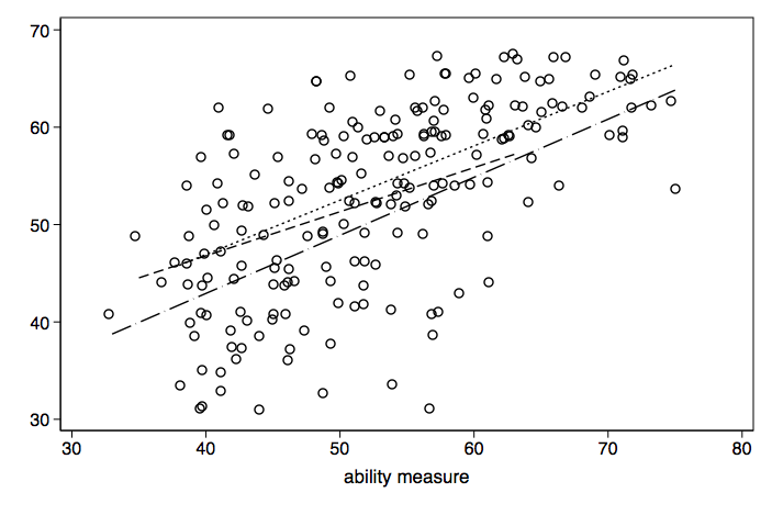
The F-ratio, F(5, 194) = 26.43, for the full model with treatment, ability, and interaction is significant, go to Step 2.

Step 2: Test interaction.

testparm treat#c.ability

 ( 1)  2.treat#c.ability = 0
 ( 2)  3.treat#c.ability = 0

       F(  2,   194) =    0.27
            Prob > F =    0.7604

The interaction is not significant, go to Step 3.

Step 3: Test common regressio, coefficient.

regress score i.treat ability

      Source |       SS       df       MS              Number of obs =     200
-------------+------------------------------           F(  3,   196) =   44.20
       Model |  7214.30058     3  2404.76686           Prob > F      =  0.0000
    Residual |  10664.5744   196   54.411094           R-squared     =  0.4035
-------------+------------------------------           Adj R-squared =  0.3944
       Total |   17878.875   199   89.843593           Root MSE      =  7.3764

------------------------------------------------------------------------------
       score |      Coef.   Std. Err.      t    P>|t|     [95% Conf. Interval]
-------------+----------------------------------------------------------------
       treat |
          2  |   1.248212   1.381794     0.90   0.367     -1.47688    3.973304
          3  |  -2.600438   1.532905    -1.70   0.091    -5.623543    .4226668
             |
     ability |   .5476883   .0635714     8.62   0.000     .4223166    .6730601
       _cons |   23.93675   3.364732     7.11   0.000     17.30102    30.57247
------------------------------------------------------------------------------

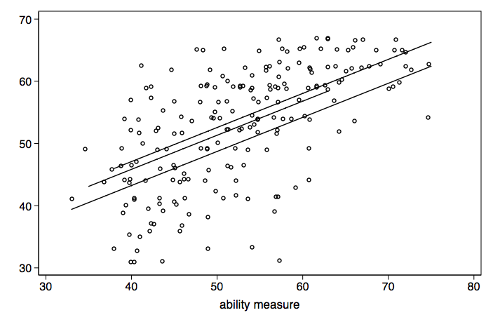
predict p2

sort treat p2

graph twoway scatter score p2 ability, s(oh i) c(. L) jitter(2) legend(off)



test ability

 ( 1)  ability = 0.0

       F(  1,   196) =   74.22
            Prob > F =    0.0000

The regression coefficient for ability is significant, go to Step 5.

Step 5: Test intercepts.

testparm i.treat

 ( 1)  2.treat = 0
 ( 2)  3.treat = 0

       F(  2,   196) =    3.66
            Prob > F =    0.0276

The treatment is significant, calculate seperate intercepts with common regression coefficient.


y' = 23.94 + 1.25(2.treat) - 2.6(3.treat) + .55(ability)
y' = 23.94 + 1.25(0)         - 2.6(0)     + .55(ability)
y' = 23.94 + .55(ability) {treatment group 1}

y' = 23.94 + 1.25(2.treat) - 2.6(3.treat) + .55(ability)
y' = 23.94 + 1.25(1)         - 2.6(0)     + .55(ability)
y' = 25.19 + .55(ability) {treatment group 2}

y' = 23.94 + 1.25(2.treat) - 2.6(3.treat) + .55(ability)
y' = 23.94 + 1.25(0)         - 2.6(1)     + .55(ability)
y' = 21.34 + .55(ability) {treatment group 3}

Linear Statistical Models Course

Phil Ender, 29Jan98