use http://www.philender.com/courses/data/hsbdemo, clear
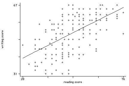
regress write read
Source | SS df MS Number of obs = 200
-------------+------------------------------ F( 1, 198) = 109.52
Model | 6367.42127 1 6367.42127 Prob > F = 0.0000
Residual | 11511.4537 198 58.1386552 R-squared = 0.3561
-------------+------------------------------ Adj R-squared = 0.3529
Total | 17878.875 199 89.843593 Root MSE = 7.6249
------------------------------------------------------------------------------
write | Coef. Std. Err. t P>|t| [95% Conf. Interval]
-------------+----------------------------------------------------------------
read | .5517051 .0527178 10.47 0.000 .4477445 .6556656
_cons | 23.95944 2.805744 8.54 0.000 18.42647 29.49242
------------------------------------------------------------------------------
twoway (scatter write read, msym(oh))(lfit write read), legend(off)
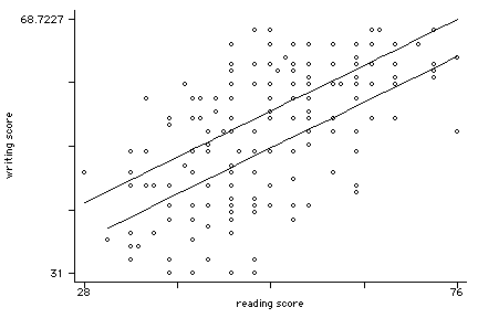
regress write read female

      Source |       SS       df       MS              Number of obs =     200
-------------+------------------------------           F(  2,   197) =   77.21
       Model |  7856.32118     2  3928.16059           Prob > F      =  0.0000
    Residual |  10022.5538   197  50.8759077           R-squared     =  0.4394
-------------+------------------------------           Adj R-squared =  0.4337
       Total |   17878.875   199   89.843593           Root MSE      =  7.1327

------------------------------------------------------------------------------
       write |      Coef.   Std. Err.      t    P>|t|     [95% Conf. Interval]
-------------+----------------------------------------------------------------
        read |   .5658869   .0493849    11.46   0.000      .468496    .6632778
      female |   5.486894   1.014261     5.41   0.000      3.48669    7.487098
       _cons |   20.22837   2.713756     7.45   0.000     14.87663    25.58011
------------------------------------------------------------------------------


predict p2
sort female p2

scatter write p2 read, msym(oh i) con(. L) sort
generate fxr = female*read
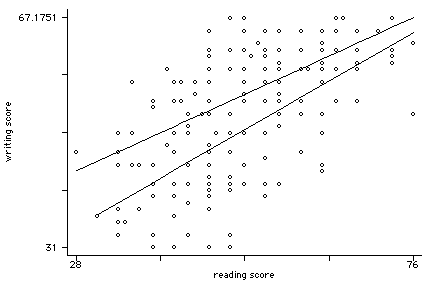
regress write c.read##i.female
Source | SS df MS Number of obs = 200
-------------+------------------------------ F( 3, 196) = 52.31
Model | 7949.6163 3 2649.8721 Prob > F = 0.0000
Residual | 9929.2587 196 50.6594831 R-squared = 0.4446
-------------+------------------------------ Adj R-squared = 0.4361
Total | 17878.875 199 89.843593 Root MSE = 7.1175
------------------------------------------------------------------------------
write | Coef. Std. Err. t P>|t| [95% Conf. Interval]
-------------+----------------------------------------------------------------
read | .6360156 .0714073 8.91 0.000 .4951904 .7768408
1.female | 12.49063 5.259266 2.37 0.019 2.118614 22.86265
|
female#|
c.read |
1 | -.133902 .0986707 -1.36 0.176 -.3284945 .0606905
|
_cons | 16.52388 3.845114 4.30 0.000 8.940769 24.10699
------------------------------------------------------------------------------
twoway (scatter write read, msym(oh)) (lfit write read if female==0) ///
(lfit write read if female==1), legend(off)xxxxxxx
Classical ANCOVA
- Partial out effects of one or more nuisance variables from the dependent variable.
- Random assignment to groups.
- One or more continuous variables.
- Statistical control vs experimental control.
Assumptions
- Independence
- Normality
- Homogeneity of variance
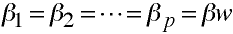
- Population within group regression coefficients are equal
- covariate is measured without error
- Regression residuals are NID with mean 0 and equal variances
- Relationship between covariate & dependent variable is linear
- Covariate is related to dependent variable but is logically independent of treatment.
Selecting a Covariate
- The experiment contains one or more extraneous sources of variation--
- Related to the dependent variable
- Irrelevant to the independent variable
- Experimental control is not feasible or possible
- If possible measure covariate so that it does not include treatment effects
- Covariate obtained prior to treatment
- Covariate obtained after treatment but before it take effect
- Covariate is assumed to be unaffected by treatment
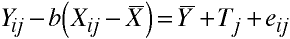
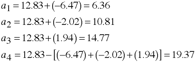
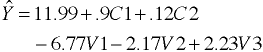
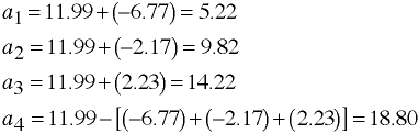
Logic of ANCOVA
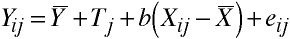
Which may be rewritten:
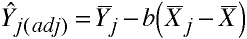
Homogeneity of Regression
- The previous two formulas involved the use of a common regression coefficient, b.
- Assumes that the slope of the regression line is constant across groups.
- Test the interaction of the independent variable and the covariate.
Steps in ANCOVA
- Include variable of scores on the dependent variable -- y
- Include variables of scores on the covariates -- c
- Create variables for coded group membership -- v
- Multiply each v by c to create interaction vectors -- cv
- Test variance added by step 4 -- homogeneity of regression slopes -- If n.s. procede to step 6; if sig. analyze as ATI
- Test variance added by step 3 -- If sig. then there are treatment effects, procede to step 7; if n.s. calculate regression with covariate only.
- If there are more than 2 levels perform multiple comparisons.
Numerical Example: coded using Effect Coding
input id  y  c1  c2 grp  v1  v2  v3
 1  6   1   6   1   1   0   0
 2  9   1   7   1   1   0   0
 3  8   2  15   1   1   0   0
 4  8   3  13   1   1   0   0
 5 12   3  18   1   1   0   0
 6 12   4   9   1   1   0   0
 7 10   4  16   1   1   0   0
 8  8   5  10   1   1   0   0
 9 12   5  16   1   1   0   0
10 13   6  18   1   1   0   0
11 13   4  12   2   0   1   0
12 16   4  12   2   0   1   0
13 15   5  17   2   0   1   0
14 16   6   9   2   0   1   0
15 19   6  20   2   0   1   0
16 17   8  18   2   0   1   0
17 19   8  16   2   0   1   0
18 23   9  20   2   0   1   0
19 19  10  10   2   0   1   0
20 22  10  17   2   0   1   0
21 20   7   8   3   0   0   1
22 22   7  14   3   0   0   1
23 24   9  11   3   0   0   1
24 26   9  11   3   0   0   1
25 24  10  16   3   0   0   1
26 25  11  20   3   0   0   1
27 28  11  19   3   0   0   1
28 27  12  19   3   0   0   1
29 29  13  12   3   0   0   1
30 26  13  16   3   0   0   1
31 27   7  16   4  -1  -1  -1
32 28   8  10   4  -1  -1  -1
33 25   8  13   4  -1  -1  -1
34 27   9   7   4  -1  -1  -1
35 31   9  15   4  -1  -1  -1
36 29  10  20   4  -1  -1  -1
37 32  10  16   4  -1  -1  -1
38 30  12  21   4  -1  -1  -1
39 32  12  15   4  -1  -1  -1
40 33  14  21   4  -1  -1  -1
end

/* using regress with factor variables */

regress y i.grp##c.c1

      Source |       SS       df       MS              Number of obs =      40
-------------+------------------------------           F(  7,    32) =  109.27
       Model |  2382.23359     7  340.319084           Prob > F      =  0.0000
    Residual |  99.6664092    32  3.11457529           R-squared     =  0.9598
-------------+------------------------------           Adj R-squared =  0.9511
       Total |      2481.9    39  63.6384615           Root MSE      =  1.7648

------------------------------------------------------------------------------
           y |      Coef.   Std. Err.      t    P>|t|     [95% Conf. Interval]
-------------+----------------------------------------------------------------
         grp |
          2  |   3.435985   2.272924     1.51   0.140     -1.19381     8.06578
          3  |   7.650473   3.069013     2.49   0.018     1.399098    13.90185
          4  |   13.34207   3.017006     4.42   0.000     7.196633    19.48752
             |
          c1 |   .9015152   .3434768     2.62   0.013     .2018757    1.601155
             |
    grp#c.c1 |
          2  |   .2026515   .4276252     0.47   0.639    -.6683925    1.073696
          3  |   .1489436   .4352144     0.34   0.734    -.7375591    1.035446
          4  |   .0402098   .4365514     0.09   0.927    -.8490164     .929436
             |
       _cons |   6.734848    1.29432     5.20   0.000     4.098405    9.371292
------------------------------------------------------------------------------

testparm grp#c.c1


 ( 1)  2.grp#c.c1 = 0
 ( 2)  3.grp#c.c1 = 0
 ( 3)  4.grp#c.c1 = 0

       F(  3,    32) =    0.11
            Prob > F =    0.9550

/* using anova */

anova y i.grp##c.c1

                           Number of obs =      40     R-squared     =  0.9598
                           Root MSE      = 1.76482     Adj R-squared =  0.9511

                  Source |  Partial SS    df       MS           F     Prob > F
              -----------+----------------------------------------------------
                   Model |  2382.23359     7  340.319084     109.27     0.0000
                         |
                     grp |  70.1635717     3  23.3878572       7.51     0.0006
                      c1 |  152.279387     1  152.279387      48.89     0.0000
                  grp#c1 |  1.00618243     3  .335394144       0.11     0.9550
                         |
                Residual |  99.6664092    32  3.11457529
              -----------+----------------------------------------------------
                   Total |      2481.9    39  63.6384615

/* without interaction */

anova y i.grp c1

                           Number of obs =      40     R-squared     =  0.9681
                           Root MSE      = 1.85482     Adj R-squared =  0.9459

                  Source |  Partial SS    df       MS           F     Prob > F
              -----------+----------------------------------------------------
                   Model |  2402.77139    16  150.173212      43.65     0.0000
                         |
                     grp |  270.804721     3  90.2682404      26.24     0.0000
                      c1 |  186.671388    13  14.3593375       4.17     0.0014
                         |
                Residual |  79.1286121    23  3.44037444
              -----------+----------------------------------------------------
                   Total |      2481.9    39  63.6384615

/* back to regress with factor variables */

regress y i.grp c1

      Source |       SS       df       MS              Number of obs =      40
-------------+------------------------------           F(  4,    35) =  206.97
       Model |  2381.22741     4  595.306852           Prob > F      =  0.0000
    Residual |  100.672592    35  2.87635976           R-squared     =  0.9594
-------------+------------------------------           Adj R-squared =  0.9548
       Total |      2481.9    39  63.6384615           Root MSE      =   1.696

------------------------------------------------------------------------------
           y |      Coef.   Std. Err.      t    P>|t|     [95% Conf. Interval]
-------------+----------------------------------------------------------------
         grp |
          2  |   4.453014   .8983061     4.96   0.000     2.629356    6.276673
          3  |   8.411249   1.184014     7.10   0.000     6.007572    10.81493
          4  |   13.01516     1.1535    11.28   0.000     10.67344    15.35689
             |
          c1 |   1.013052   .1337037     7.58   0.000     .7416185    1.284485
       _cons |   6.355625    .703058     9.04   0.000     4.928341    7.782908
------------------------------------------------------------------------------

testparm i.grp

 ( 1)  2.grp = 0
 ( 2)  3.grp = 0
 ( 3)  4.grp = 0

       F(  3,    35) =   48.19
            Prob > F =    0.0000

/* compute original means */

table grp, contents(mean y)

----------+-----------
      grp |    mean(y)
----------+-----------
        1 |        9.8
        2 |       17.9
        3 |       25.1
        4 |       29.4
----------+-----------

/* compute adjusted means using margins */
/* margins will work with either regress or anova */

margins grp, asbalanced

Predictive margins                                Number of obs   =         40
Model VCE    : OLS

Expression   : Linear prediction, predict()

------------------------------------------------------------------------------
             |            Delta-method
             |     Margin   Std. Err.      z    P>|z|     [95% Conf. Interval]
-------------+----------------------------------------------------------------
         grp |
          1  |   14.08014   .7789391    18.08   0.000     12.55345    15.60684
          2  |   18.53316   .5427882    34.14   0.000     17.46931      19.597
          3  |   22.49139   .6373144    35.29   0.000     21.24228    23.74051
          4  |   27.09531   .6165704    43.95   0.000     25.88685    28.30376
------------------------------------------------------------------------------
Regression Equation

Separate Intercepts
Computing Adjusted Means
Multiple Covariates
- Effects of two or more covariates are removed from the dependent variable.
- Proceeds in a manner similar to the single covariate model.
Numerical Example
Same data as above example, except for the additional interaction terms:

/* run regression */

regress y c.c1##grp c.c2##grp

      Source |       SS       df       MS              Number of obs =      40
-------------+------------------------------           F( 11,    28) =   71.35
       Model |  2396.40189    11  217.854717           Prob > F      =  0.0000
    Residual |  85.4981125    28  3.05350402           R-squared     =  0.9656
-------------+------------------------------           Adj R-squared =  0.9520
       Total |      2481.9    39  63.6384615           Root MSE      =  1.7474

------------------------------------------------------------------------------
           y |      Coef.   Std. Err.      t    P>|t|     [95% Conf. Interval]
-------------+----------------------------------------------------------------
          c1 |   .6228412   .4106184     1.52   0.141    -.2182726    1.463955
             |
         grp |
          2  |   1.748814   3.135003     0.56   0.581    -4.672948    8.170576
          3  |   9.113772   3.358697     2.71   0.011     2.233793    15.99375
          4  |   14.68458   3.254535     4.51   0.000     8.017967    21.35119
             |
    grp#c.c1 |
          2  |   .3730242   .4858476     0.77   0.449    -.6221895    1.368238
          3  |   .4238656    .517841     0.82   0.420    -.6368836    1.484615
          4  |   .2512126   .5316271     0.47   0.640    -.8377761    1.340201
             |
          c2 |   .1896132   .1565606     1.21   0.236    -.1310866    .5103131
             |
    grp#c.c2 |
          2  |   .0703098   .2157489     0.33   0.747    -.3716317    .5122513
          3  |  -.1858784   .2318612    -0.80   0.429    -.6608245    .2890676
          4  |  -.1372108   .2240572    -0.61   0.545    -.5961711    .3217495
             |
       _cons |   5.255291   1.770547     2.97   0.006      1.62849    8.882092
------------------------------------------------------------------------------

/* test homogeneity of regression slopes */

testparm grp#c.c1 grp#c.c2


 ( 1)  2.grp#c.c1 = 0
 ( 2)  3.grp#c.c1 = 0
 ( 3)  4.grp#c.c1 = 0
 ( 4)  2.grp#c.c2 = 0
 ( 5)  3.grp#c.c2 = 0
 ( 6)  4.grp#c.c2 = 0

       F(  6,    28) =    0.43
            Prob > F =    0.8553

/* using anova */

 anova y c.c1##grp c.c2##grp

                            Number of obs =      40     R-squared     =  0.9656
                           Root MSE      = 1.74743     Adj R-squared =  0.9520

                  Source |  Partial SS    df       MS           F     Prob > F
              -----------+----------------------------------------------------
                   Model |  2396.40189    11  217.854717      71.35     0.0000
                         |
                      c1 |  85.0803048     1  85.0803048      27.86     0.0000
                     grp |  73.5988644     3  24.5329548       8.03     0.0005
                  grp#c1 |  2.40458727     3   .80152909       0.26     0.8518
                      c2 |  7.69362841     1  7.69362841       2.52     0.1237
                  grp#c2 |  5.14302215     3  1.71434072       0.56     0.6449
                         |
                Residual |  85.4981125    28  3.05350402
              -----------+----------------------------------------------------
                   Total |      2481.9    39  63.6384615

test grp#c.c1 grp#c.c2

                  Source |  Partial SS    df       MS           F     Prob > F
           --------------+----------------------------------------------------
           grp#c1 grp#c2 |  7.80432184     6  1.30072031       0.43     0.8553
                Residual |  85.4981125    28  3.05350402

/* anova without interaction */

anova y c.c1 c.c2 grp

                           Number of obs =      40     R-squared     =  0.9624
                           Root MSE      = 1.65656     Adj R-squared =  0.9569

                  Source |  Partial SS    df       MS           F     Prob > F
              -----------+----------------------------------------------------
                   Model |  2388.59757     5  477.719513     174.08     0.0000
                         |
                      c1 |   98.974038     1   98.974038      36.07     0.0000
                      c2 |  7.37015734     1  7.37015734       2.69     0.1105
                     grp |  420.189396     3  140.063132      51.04     0.0000
                         |
                Residual |  93.3024343    34  2.74418925
              -----------+----------------------------------------------------
                   Total |      2481.9    39  63.6384615


/* rerun as regression */

regress

      Source |       SS       df       MS              Number of obs =      40
-------------+------------------------------           F(  5,    34) =  174.08
       Model |  2388.59757     5  477.719513           Prob > F      =  0.0000
    Residual |  93.3024343    34  2.74418925           R-squared     =  0.9624
-------------+------------------------------           Adj R-squared =  0.9569
       Total |      2481.9    39  63.6384615           Root MSE      =  1.6566

------------------------------------------------------------------------------
           y |      Coef.   Std. Err.      t    P>|t|     [95% Conf. Interval]
-------------+----------------------------------------------------------------
          c1 |   .8952525   .1490706     6.01   0.000     .5923047      1.1982
          c2 |   .1199612   .0731997     1.64   0.110    -.0287985    .2687209
             |
         grp |
          2  |    4.60118   .8820702     5.22   0.000     2.808598    6.393762
          3  |   8.996353   1.210347     7.43   0.000     6.536631    11.45607
          4  |   13.46896   1.160214    11.61   0.000     11.11112     15.8268
             |
       _cons |   5.220638   .9753057     5.35   0.000     3.238579    7.202698
------------------------------------------------------------------------------

/* compute original means again */
table grp, contents(mean y)

----------+-----------
      grp |    mean(y)
----------+-----------
        1 |        9.8
        2 |       17.9
        3 |       25.1
        4 |       29.4
----------+-----------

/* compute adjusted means using margins */

margins grp, asbalanced

Predictive margins                                Number of obs   =         40

Expression   : Linear prediction, predict()

------------------------------------------------------------------------------
             |            Delta-method
             |     Margin   Std. Err.      z    P>|z|     [95% Conf. Interval]
-------------+----------------------------------------------------------------
         grp |
          1  |   13.78338   .7820854    17.62   0.000     12.25052    15.31624
          2  |   18.38456    .537869    34.18   0.000     17.33035    19.43876
          3  |   22.77973    .646886    35.21   0.000     21.51186     24.0476
          4  |   27.25234   .6098128    44.69   0.000     26.05713    28.44755
------------------------------------------------------------------------------
Regression Equation
Separate Intercepts
Interpretational Problems
- ANCOVA in experimental vs quasi-experimental research.
- "Equating" intact groups.
- "...what exactly does it mean to ask what the data would look like if they were not as they are" (Anderson, 1963).
- Lord, 1969-
- Controling for height of plant.
- What would be the yield of a 6ft variety be if they were 7ft?
- Depends on how you make them taller.
Specification Error
- Many problems in equating nonequivalent groups using ANCOVA are due to specification error.
- Can lead to over- or underadjustment of treatment means.
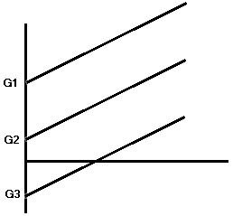
Extrapolation Errors
- When there is little or no overlap in group distributions
- Regression line for lowest group extrapolated upwards-
- Regression line for highest group extrapolated downwards.
Differential Growth
- Control using pretest as covariate
- Assumes rate of growth in nonequivalent groups are equal.
- Can lead to situations where differences in adjusted scores is due to differential growth.
Nonlinearity
- Do not assume that the regression is linear. Study the shape of the relationship. Avoiding erroneous assumptions and inappropriate analyses.
Measurement Error
- Measurement error in the covariate:
- Leads to underestimation of regression coefficient.
- This leads to underadjustment in the group lower on the CV.
- Often the treatment group in social intervention research.
Stata Example
These data are from a 1996 study (Gregoire, Kumar, Everitt, Henderson & Studd; also in Rabe-Hesketh & Everitt, 1999) on the efficacy of estrogen patches in treating postpartum depression. Women were randomly assigned to either a placebo control group (group=0, n=27) or estrogen patch group (group=1, n=34). Prior to the first treatment all patients took the Edinburgh Postnatal Depression Scale (EPDS). EPDS data was collected monthly for six months once the treatment began and average depression scores computed for each subject. Higher scores on the EDPS are indicative of higher levels of dsepression.
use http://www.philender.com/courses/data/depress1, clear

describe

Contains data from depress1.dta
  obs:            61
 vars:             4                          18 Feb 2000 11:21
 size:         1,220 (99.8% of memory free)
-------------------------------------------------------------------------------
   1. subj      float  %9.0g
   2. dep       float  %9.0g                  post-treatment depression score
   3. pre       float  %9.0g                  pre-treatment depression score
   4. group     float  %14.0g      gl         treatment group
-------------------------------------------------------------------------------

codebook group

group --------------------------------------------------------- treatment group
                  type:  numeric (float)
                 label:  gl

                 range:  [0,1]                        units:  1
         unique values:  2                    coded missing:  0 / 61

            tabulation:  Freq.   Numeric  Label
                            27         0  placebo patch
                            34         1  estrogen patch

summarize pre dep

Variable |     Obs        Mean   Std. Dev.       Min        Max
---------+-----------------------------------------------------
     pre |      61    21.04033   3.722975         15         28
     dep |      61    12.41284   5.407777          2       26.5

ttest pre, by(group)

Two-sample t test with equal variances

------------------------------------------------------------------------------
   Group |     Obs        Mean    Std. Err.   Std. Dev.   [95% Conf. Interval]
---------+--------------------------------------------------------------------
placebo  |      27    20.77778    .7611158    3.954874    19.21328    22.34227
estrogen |      34    21.24882      .61301    3.574432    20.00165      22.496
---------+--------------------------------------------------------------------
combined |      61    21.04033     .476678    3.722975    20.08683    21.99383
---------+--------------------------------------------------------------------
    diff |           -.4710457    .9658499               -2.403707    1.461615
------------------------------------------------------------------------------
Degrees of freedom: 59

               Ho: mean(placebo ) - mean(estrogen) = diff = 0

     Ha: diff < 0               Ha: diff ~= 0              Ha: diff > 0
       t =  -0.4877                t =  -0.4877              t =  -0.4877
   P < t =   0.3138          P > |t| =   0.6276          P > t =   0.6862

pwcorr dep pre, sig

             |      dep      pre
-------------+------------------
         dep |   1.0000
             |
             |
         pre |   0.2920   1.0000
             |   0.0224
             |

/* a quick-and-dirty scatterplot  */

plot dep pre

   26.5 +
    p    |                                                                 *
    o    |
    s    |                                                       *
    t    |                                                              *
    -    |     *
    t    |
    r    |               *
    e    |                    *    *    *    *                   *    *
    a    |                                   *              *              *
    t    |     *    *    *              *    *                   *
    m    |                                        *    *
    e    | *                                           *    *
    n    |                    *              *
    t    |     *    *              *    *                        *    *
         | *   *
    d    | *                  *    *              *
    e    |               *              *         *
    p    |               *         *         *
    r    |          *                   *                                  *
       2 +               *         *
          +----------------------------------------------------------------+
               15         pre-treatment depression score               28

/* analysis without covariate  */

regress dep i.group


      Source |       SS       df       MS              Number of obs =      61
-------------+------------------------------           F(  1,    59) =   10.54
       Model |  265.972224     1  265.972224           Prob > F      =  0.0019
    Residual |  1488.67078    59  25.2317081           R-squared     =  0.1516
-------------+------------------------------           Adj R-squared =  0.1372
       Total |    1754.643    60  29.2440501           Root MSE      =  5.0231

------------------------------------------------------------------------------
         dep |      Coef.   Std. Err.      t    P>|t|     [95% Conf. Interval]
-------------+----------------------------------------------------------------
     1.group |   -4.20399   1.294842    -3.25   0.002    -6.794964   -1.613017
       _cons |   14.75605   .9666994    15.26   0.000     12.82169    16.69041
------------------------------------------------------------------------------

margins group, asbalanced

Adjusted predictions                              Number of obs   =         61
Model VCE    : OLS

Expression   : Linear prediction, predict()

------------------------------------------------------------------------------
             |            Delta-method
             |     Margin   Std. Err.      z    P>|z|     [95% Conf. Interval]
-------------+----------------------------------------------------------------
       group |
          0  |   14.75605   .9666994    15.26   0.000     12.86135    16.65075
          1  |   10.55206   .8614575    12.25   0.000     8.863633    12.24048
------------------------------------------------------------------------------
The ANCOVA
/* test for treat by covariate interation */

anova dep c.pre##group

                           Number of obs =      61     R-squared     =  0.2541
                           Root MSE      = 4.79187     Adj R-squared =  0.2148

                  Source |  Partial SS    df       MS           F     Prob > F
              -----------+----------------------------------------------------
                   Model |   445.80933     3   148.60311       6.47     0.0008
                         |
                     pre |  177.442758     1  177.442758       7.73     0.0074
                   group |  1.49167086     1  1.49167086       0.06     0.7997
               group#pre |  3.19588284     1  3.19588284       0.14     0.7105
                         |
                Residual |  1308.83367    57  22.9619943
              -----------+----------------------------------------------------
                   Total |    1754.643    60  29.2440501

regress dep pre i.group

      Source |       SS       df       MS              Number of obs =      61
-------------+------------------------------           F(  2,    58) =    9.78
       Model |  442.613448     2  221.306724           Prob > F      =  0.0002
    Residual |  1312.02956    58  22.6211993           R-squared     =  0.2523
-------------+------------------------------           Adj R-squared =  0.2265
       Total |    1754.643    60  29.2440501           Root MSE      =  4.7562

------------------------------------------------------------------------------
         dep |      Coef.   Std. Err.      t    P>|t|     [95% Conf. Interval]
-------------+----------------------------------------------------------------
         pre |   .4618001   .1652592     2.79   0.007     .1309977    .7926024
     1.group |  -4.421519     1.2285    -3.60   0.001    -6.880629    -1.96241
       _cons |    5.16087   3.553626     1.45   0.152    -1.952484    12.27422
------------------------------------------------------------------------------

table group, contents(mean dep)

---------------+-----------
treatment      |
group          |  mean(dep)
---------------+-----------
 placebo patch |   14.75605
estrogen patch |   10.55206
---------------+-----------

margins group, asbalanced

Predictive margins                                Number of obs   =         61
Model VCE    : OLS

Expression   : Linear prediction, predict()

------------------------------------------------------------------------------
             |            Delta-method
             |     Margin   Std. Err.      z    P>|z|     [95% Conf. Interval]
-------------+----------------------------------------------------------------
       group |
          0  |   14.87729   .9163541    16.24   0.000     13.08127    16.67332
          1  |   10.45578   .8164047    12.81   0.000     8.855652     12.0559
------------------------------------------------------------------------------
Interpretation
The interaction between the covariate (pre) and the treatment (group) was not significant, implying that we have homogeneity of regression slopes. In the final regression model, both the covariate and the treatment were statistically significant. Women with higher pretest scores on depression remain higher after treatment. Each point increase on the pretest was associated with about a .46 point increase on the predicted posttest score.
The effect of the estrogen patch was also significant. Women using the treatment patch had predicted depression scoress almost 4.5 points lower than women using the control patch.
Another Stata Example
These data examine a reading instruction program called "reading recovery." Students are randomly assigned to two treatment groups: a control group which receives standard reading instruction (treat = 0, n = 43) and the reading recovery group (treat = 1, n = 32).
There were two pretests administered at the beginning of the year. One test (pre1) consisted of dictation tasks, and the second (pre2) were early literacy skills. After four months of remedial reading instruction, the students we administered a standardized test of reading skills.
We will begin be examining the variables and determining if the treatment groups differ on the pretest measures.
use http://www.philender.com/courses/data/readexp, clear

describe

Contains data from readexp.dta
  obs:            75
 vars:             6                          21 Dec 2000 21:29
 size:         2,100 (99.8% of memory free)
-------------------------------------------------------------------------------
   1. id        float  %9.0g
   2. school    float  %9.0g
   3. treat     float  %9.0g
   4. pre1      float  %9.0g
   5. pre2      float  %9.0g
   6. post      float  %9.0g
-------------------------------------------------------------------------------

tabulate treat

      treat |      Freq.     Percent        Cum.
------------+-----------------------------------
          0 |         43       57.33       57.33
          1 |         32       42.67      100.00
------------+-----------------------------------
      Total |         75      100.00

summarize pre1 pre2 post

Variable |     Obs        Mean   Std. Dev.       Min        Max
---------+-----------------------------------------------------
    pre1 |      75        8.44   7.571711          0         31
    pre2 |      75    39.05333   18.32506          7         88
    post |      75    33.26667   11.11528         12         64

corr pre1 pre2 post
(obs=75)

         |     pre1     pre2     post
---------+---------------------------
    pre1 |   1.0000
    pre2 |   0.6017   1.0000
    post |   0.3202   0.5522   1.0000

stem pre1 if treat==0, lines(2)

Stem-and-leaf plot for pre1

  0* | 00001222333344444
  0. | 555667789
  1* | 0134
  1. | 568899
  2* | 013
  2. | 569
  3* | 1

stem pre1 if treat==1, lines(2)

Stem-and-leaf plot for pre1

  0* | 0001222223344
  0. | 5556678889
  1* | 000111
  1. | 66
  2* | 1

stem pre2 if treat==0, lines(1)

Stem-and-leaf plot for pre2

  0* | 7
  1* | 0668889
  2* | 0013356899
  3* | 0146789
  4* | 13346
  5* | 01225679
  6* | 1366
  7* |
  8* | 8

stem pre2 if treat==1, lines(1)

Stem-and-leaf plot for pre2

  0* | 9
  1* | 367
  2* | 12379
  3* | 02358
  4* | 001677
  5* | 00123469
  6* | 17
  7* |
  8* | 24


ttest pre1, by(treat)

Two-sample t test with equal variances

------------------------------------------------------------------------------
   Group |     Obs        Mean    Std. Err.   Std. Dev.   [95% Conf. Interval]
---------+--------------------------------------------------------------------
       0 |      43    9.883721    1.337014    8.767389    7.185517    12.58192
       1 |      32         6.5    .9002688    5.092689     4.66389     8.33611
---------+--------------------------------------------------------------------
combined |      75        8.44    .8743059    7.571711    6.697908    10.18209
---------+--------------------------------------------------------------------
    diff |            3.383721    1.735173               -.0744738    6.841916
------------------------------------------------------------------------------
Degrees of freedom: 73

                      Ho: mean(0) - mean(1) = diff = 0

     Ha: diff < 0               Ha: diff ~= 0              Ha: diff > 0
       t =   1.9501                t =   1.9501              t =   1.9501
   P < t =   0.9725          P > |t| =   0.0550          P > t =   0.0275

ttest pre2, by(treat)

Two-sample t test with equal variances

------------------------------------------------------------------------------
   Group |     Obs        Mean    Std. Err.   Std. Dev.   [95% Conf. Interval]
---------+--------------------------------------------------------------------
       0 |      43    37.30233    2.769381    18.16005    31.71349    42.89116
       1 |      32    41.40625    3.282671    18.56959     34.7112     48.1013
---------+--------------------------------------------------------------------
combined |      75    39.05333    2.115996    18.32506    34.83712    43.26955
---------+--------------------------------------------------------------------
    diff |           -4.103924    4.280596               -12.63514    4.427291
------------------------------------------------------------------------------
Degrees of freedom: 73

                      Ho: mean(0) - mean(1) = diff = 0

     Ha: diff < 0               Ha: diff ~= 0              Ha: diff > 0
       t =  -0.9587                t =  -0.9587              t =  -0.9587
   P < t =   0.1704          P > |t| =   0.3409          P > t =   0.8296

ranksum pre1, by(treat)

Two-sample Wilcoxon rank-sum (Mann-Whitney) test

   treat |      obs    rank sum    expected
---------+---------------------------------
       0 |       43        1748        1634
       1 |       32        1102        1216
---------+---------------------------------
combined |       75        2850        2850

unadjusted variance     8714.67
adjustment for ties      -39.54
                     ----------
adjusted variance       8675.12

Ho: pre1(treat==0) = pre1(treat==1)
             z =   1.224
    Prob > |z| =   0.2210

ranksum pre2, by(treat)

Two-sample Wilcoxon rank-sum (Mann-Whitney) test

   treat |      obs    rank sum    expected
---------+---------------------------------
       0 |       43      1547.5        1634
       1 |       32      1302.5        1216
---------+---------------------------------
combined |       75        2850        2850

unadjusted variance     8714.67
adjustment for ties       -4.71
                     ----------
adjusted variance       8709.96

Ho: pre2(treat==0) = pre2(treat==1)
             z =  -0.927
    Prob > |z| =   0.3540
Interpretation
Because there appears to be a great deal of skewness in pre2 and some differences in the shapes of the distributions for pre1 Mann-Whitney tests (ranksum command) are preferable to the Student's t-tests for looking at pretest differences in the groups
Now, let's conduct the analysis of covariance.
/* without covariates */

regress post treat

  Source |       SS       df       MS                  Number of obs =      75
---------+------------------------------               F(  1,    73) =    8.39
   Model |  942.050388     1  942.050388               Prob > F      =  0.0050
Residual |  8200.61628    73  112.337209               R-squared     =  0.1030
---------+------------------------------               Adj R-squared =  0.0908
   Total |  9142.66667    74   123.54955               Root MSE      =  10.599

------------------------------------------------------------------------------
    post |      Coef.   Std. Err.       t     P>|t|       [95% Conf. Interval]
---------+--------------------------------------------------------------------
   treat |   7.165698   2.474476      2.896   0.005       2.234075    12.09732
   _cons |    30.2093   1.616321     18.690   0.000       26.98798    33.43063
------------------------------------------------------------------------------

/* test treatment by slope interaction */

anova post c.pre1##treat c.pre2##treat

                           Number of obs =      75     R-squared     =  0.3989
                           Root MSE      = 8.92437     Adj R-squared =  0.3554

                  Source |  Partial SS    df       MS           F     Prob > F
              -----------+----------------------------------------------------
                   Model |  3647.21028     5  729.442056       9.16     0.0000
                         |
                    pre1 |   .66873253     1   .66873253       0.01     0.9273
                   treat |  22.9971541     1  22.9971541       0.29     0.5928
              treat#pre1 |  137.179391     1  137.179391       1.72     0.1937
                    pre2 |  1190.78252     1  1190.78252      14.95     0.0002
              treat#pre2 |  144.906484     1  144.906484       1.82     0.1818
                         |
                Residual |  5495.45639    69  79.6442955
              -----------+----------------------------------------------------
                   Total |  9142.66667    74   123.54955

test treat#c.pre1 treat#c.pre2

                  Source |  Partial SS    df       MS           F     Prob > F
   ----------------------+----------------------------------------------------
   treat#pre1 treat#pre2 |  168.245679     2  84.1228394       1.06     0.3533
                Residual |  5495.45639    69  79.6442955


/* the ancova */

regress post pre1 pre2 i.treat

      Source |       SS       df       MS              Number of obs =      75
-------------+------------------------------           F(  3,    71) =   14.54
       Model |   3478.9646     3  1159.65487           Prob > F      =  0.0000
    Residual |  5663.70207    71  79.7704516           R-squared     =  0.3805
-------------+------------------------------           Adj R-squared =  0.3543
       Total |  9142.66667    74   123.54955           Root MSE      =  8.9314

------------------------------------------------------------------------------
        post |      Coef.   Std. Err.      t    P>|t|     [95% Conf. Interval]
-------------+----------------------------------------------------------------
        pre1 |   .1698471   .1843945     0.92   0.360    -.1978251    .5375193
        pre2 |   .2726797   .0747458     3.65   0.001     .1236409    .4217185
     1.treat |   6.621356   2.253639     2.94   0.004     2.127727    11.11499
       _cons |   18.35899   2.525568     7.27   0.000     13.32315    23.39483
------------------------------------------------------------------------------

regress post pre2 i.treat

      Source |       SS       df       MS              Number of obs =      75
-------------+------------------------------           F(  2,    72) =   21.43
       Model |  3411.28428     2  1705.64214           Prob > F      =  0.0000
    Residual |  5731.38239    72  79.6025332           R-squared     =  0.3731
-------------+------------------------------           Adj R-squared =  0.3557
       Total |  9142.66667    74   123.54955           Root MSE      =   8.922

------------------------------------------------------------------------------
        post |      Coef.   Std. Err.      t    P>|t|     [95% Conf. Interval]
-------------+----------------------------------------------------------------
        pre2 |   .3172027   .0569533     5.57   0.000     .2036683    .4307371
     1.treat |   5.863922   2.096051     2.80   0.007      1.68552    10.04232
       _cons |    18.3769   2.522833     7.28   0.000     13.34773    23.40608
------------------------------------------------------------------------------

/* unadjusted means */

tabstat post, by(treat)

Summary for variables: post
     by categories of: treat

   treat |      mean
---------+----------
       0 |   30.2093
       1 |    37.375
---------+----------
   Total |  33.26667
--------------------

margins treat, asbalanced

Predictive margins                                Number of obs   =         75
Model VCE    : OLS

Expression   : Linear prediction, predict()

------------------------------------------------------------------------------
             |            Delta-method
             |     Margin   Std. Err.      z    P>|z|     [95% Conf. Interval]
-------------+----------------------------------------------------------------
       treat |
          0  |   30.76473   1.364246    22.55   0.000     28.09085     33.4386
          1  |   36.62865   1.582889    23.14   0.000     33.52624    39.73105
------------------------------------------------------------------------------
Interpretation
The interaction between the covariates (pre1 & pre2) and the treatment (treat) were not significant, implying that we have homogeneity of regression slopes. In the regression model with no interactions pre1 was not significant and was dropped from the analysis. Both the covariate (pre2) and the treatment were statistically significant. Students with higher pretest scores on tended to have higher posttest scores. Each point increase on the pre2 was associated with about a .32 point increase on the predicted posttest score.
The effect of the reading recovery was also significant while controling for the initial level of pre2. Students receiving the treatment had predicted posttest scores almost 5.9 points higher than students in the control group. The predicted change without the covariate was approximately 7.2 points. Including the covariate reduced the amount of predicted change.
Linear Statistical Models Course
Phil Ender, 24sep10, 22Feb00