Variance & Covariance

Linear Statistical Models: Regression

Variance, Covariance & Correlation

Variance/Standard Deviation

Standard Deviation

Covariance

Another Look at Covariance

Consider the variance as being the covariance of a variable with itself.

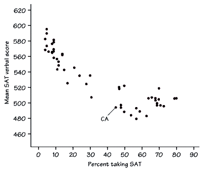
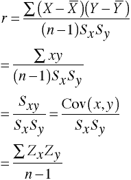
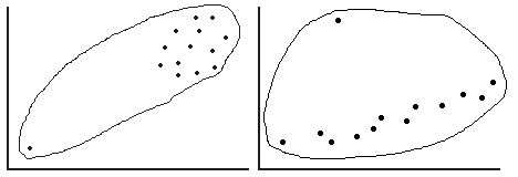
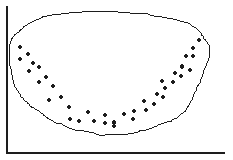
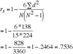
Plotting Two Variables Simultaneously

The more tightly the points are clustered together the higher the correlation between the two variables and the higher the ability to predict one variable from another.

Selected Scatter Plots

Pearson Product Moment Correlation Coefficient

Also known as, the Pearson correlation coefficient, or just the correlation coefficient.

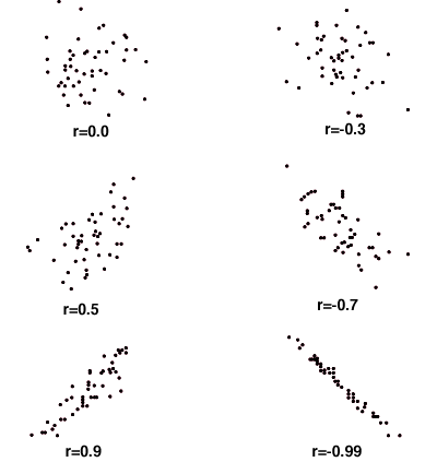
Correlation coefficients can take on any value between -1 and +1, with + and - 1 representing perfect correlations between the variables. And a correlation of zero representing no relationship between the variables.

A rule of thumb for interpreting correlation coefficients:

 Corr     Interpretation
 0 to .1  trivial
.1 to .3  small
.3 to .5  moderate
.5 to .7  large
.7 to .9  very large

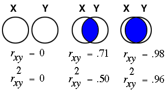
Correlations are interpreted by squaring the value of the correlation coefficient. The squared value represents the proportion of variance of one variace that is shared with the other variable, in other words, the proportion of the variance of one variable that can be predicted from the other variable.

Percent of Variance Accounted For

Correlation and Sample Size

The computation of correlation coefficients do not lend themselves to small sample sizes. The following table gives the recommended sample size for detecting various correlations with a power = 0.8 with an alpha = 0.05.

Population Correlation Coefficient

Sample Correlation Coefficient

Sources of Misleading Correlation Coefficients

Restriction of Range

Extreme Groups

Combining Groups

Outliers

Curvilinearity

Restriction of Range

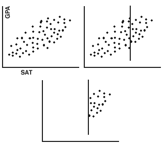
Extreme Groups

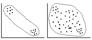
Combining Groups

Outliers

Curvilinearity

Discuss Correlation & Causation

Of course, just because two variables are correlated it does not mean that they are causally related. Often a third variable, a lurking variable, that is not included in the analysis is responsible (causes) for the first two variables. A lurking variable is a variable that loiters in the background and affects both of the original variables

Other Correlation Coefficients

Spearman rank-order correlation coefficient -- Spearman ρ

Used when data are ordinal. Interpreted like a Pearson correlation.

Eta coefficient -- η

Indicates the degree of relationship between two variables even if the relationships is nonlinear.

Eta-squared coefficient -- η²

Biserial correlation coefficient -- r_bi

For use when one variable is continuous and the other is a dichotomous variable that reflects an underlying normal distribution.

Point biserial coefficient -- r_pb

For use when one variable is continuous and the other is a 'true' dichotomous variable.

Phi coefficient -- φ

φ = (a*d - b*c)/sqrt(a*b*c*d)

Tetrachoric correlation coefficient -- r_tet

For use with two artificial dichotomous variables with underlying normal distributions.

Multiple correlation coefficient -- R_a.bcd

The correlation between a and the set of variables b, c, and d.

Squared multiple correlation coefficient - Coefficient of Determination -- R²_a.bcd

The squared correlation between a and the set of variables b, c, and d. It represents the proportion of variability of a that is accounted for by the combination of b, c, and d.

Partial correlation coefficient -- r_ab.c

The correlation between a and b with variable c partialed out. Partial correlations are useful in interpreting regression models. Spearman's Rank Order Correlation

A bivariate correlation for use when data are ranked data for both variables.

Ranked data are scaled as ordinal data.

Use Spearman's correlation, r_s (ρ).

Spearman Example

Sub xrank yrank d d²
a 1 3 -2 4
b 4 4 0 0
c 5 8 -3 9
d 10 5 5 25
e 8 2 6 36
f 14 15 -1 1
g 7 9 -2 4
h 2 6 -4 16
i 12 14 -2 4
j 9 7 2 4
k 15 13 2 4
l 3 1 2 4
m 13 12 1 1
n 11 10 1 1
o 6 11 -5 25
Sum 0 138

Stata Example

input xrank yrank
 1  3
 4  4
 5  8
10  5
 8  2
14 15
 7  9
 2  6
12 14
 9  7
15 13
 3  1
13 12
11 10
 6 11
end

corr
(obs=15)

         |    xrank    yrank
---------+------------------
   xrank |   1.0000
   yrank |   0.7536   1.0000

Another Stata Example

Now, let's use Stata to create rank data and compare the Pearson correlation with the Spearman correlation.

input y x
100 135
120 105
160 155
220 175 
110 105 
140 145 
200 185 
260 195
130 145 
110 105 
180 175 
210 165 
200 175 
170 145
120 145
end

egen xrank = rank(x)

egen yrank = rank(y)

list

             y          x      xrank      yrank 
  1.       100        135          4          1  
  2.       110        105          2        2.5  
  3.       110        105          2        2.5  
  4.       120        145        6.5        4.5  
  5.       120        105          2        4.5  
  6.       130        145        6.5          6  
  7.       140        145        6.5          7  
  8.       160        155          9          8  
  9.       170        145        6.5          9  
 10.       180        175         12         10  
 11.       200        185         14       11.5  
 12.       200        175         12       11.5  
 13.       210        165         10         13  
 14.       220        175         12         14  
 15.       260        195         15         15 

corr x y xrank yrank
(obs=15)

         |        y        x    xrank    yrank
---------+------------------------------------
       y |   1.0000
       x |   0.8768   1.0000
   xrank |   0.9118   0.9853   1.0000
   yrank |   0.9821   0.8753   0.9073   1.0000                                    

spearman x y

 Number of obs =      15
Spearman's rho =       0.9073

Test of Ho: x and y independent
      Pr > |t| =       0.0000

Point Biserial Correlation

A bivariate correlation for use when one variable is continuous and the other variable is a "true" dichotomous variable.

Point Biserial Example

input y x
100 0
120 1 
160 0 
220 1 
110 0 
140 0 
200 1 
260 1 
130 0 
110 1 
180 0 
210 1 
200 1 
170 1
120 0
end

corr x y
(obs=15)

         |        x        y
---------+------------------
       x |   1.0000
       y |   0.5541   1.0000

Fourfold Correlation - Phi Coefficient

A bivariate correlation for use when both variables are dichotomous.

Y

1 0
X 1 (a) 12 (b) 16
0 (c) 14 (d) 9

Stata Example

Use the dichotomous data with any Pearson correlation program and obtain the same correlation.

input x y w
0 0 9
0 1 14
1 0 16
1 1 12
end

corr x y [fw=w]
(obs=51)

         |        x        y
---------+------------------
       x |   1.0000
       y |  -0.1793   1.0000

Or, use the tabulate command.

tab x y [fw=w], all

           |           y
         x |         0          1 |     Total
-----------+----------------------+----------
         0 |         9         14 |        23 
         1 |        16         12 |        28 
-----------+----------------------+----------
     Total |        25         26 |        51 

          Pearson chi2(1) =   1.6394   Pr = 0.200
 likelihood-ratio chi2(1) =   1.6495   Pr = 0.199
               Cramer's V =  -0.1793
                    gamma =  -0.3494  ASE = 0.252
          Kendall's tau-b =  -0.1793  ASE = 0.138

When analyzing two-by-two tables, the value of Cramer's V is actually phi. Cramer's V is a generalization of the phi coefficient that can be used in tables larger than two-by-two.

Linear Statistical Models Course

Phil Ender, 15Jan98

Sub	xrank	yrank	d	d²
a	1	3	-2	4
b	4	4	0	0
c	5	8	-3	9
d	10	5	5	25
e	8	2	6	36
f	14	15	-1	1
g	7	9	-2	4
h	2	6	-4	16
i	12	14	-2	4
j	9	7	2	4
k	15	13	2	4
l	3	1	2	4
m	13	12	1	1
n	11	10	1	1
o	6	11	-5	25
Sum			0	138