 . That is, the constant
in the regression model is
a mean, in particular, in an intercept only model the constant is the mean
of the response variable.
. That is, the constant
in the regression model is
a mean, in particular, in an intercept only model the constant is the mean
of the response variable.At first glance, it doesn't seem that studying regression without predictors would be very useful. Certainly, we are not suggesting that using regression without predictors is a major data analysis tool. We do think that it is worthwhile to look at regression models without predictors to see what they can tell us about the nature of the constant. Understanding the regression constant in these simpler models will help us to understand both the constant and the other regression coefficients in later more complex models.
The regression constant is also known as the intercept thus, regression models without predictors are also known as intercept only models. As such, we will begin with intercept only models for OLS regression and then move on to logistic regression models without predictors.
About the data
In this section we will use a sample of 200 observations taken from the High School and Beyond (HSB) study (1986). We have selected the variable write as our response or dependent variable. The values of write represent standardized writing test scores from a test that was normalized to have a mean equal to 50 and standard deviation of 10. The table below gives the summary statistics for write.
univar write
                                        -------------- Quantiles --------------
Variable       n     Mean     S.D.      Min      .25      Mdn      .75      Max
-------------------------------------------------------------------------------
   write     200    52.77     9.48    31.00    45.50    54.00    60.00    67.00
-------------------------------------------------------------------------------
OLS regression without predictorsRegression models are designed to estimate the expected mean of a response (dependent) variable conditional on values of a set of predictor variables. An ordinary least square regression equation with a single predictor variable can be written as,
where Y is the response variable, X is a predictor variable and ε is the residual or error. The coefficient b is the regression slope coefficient and a is the constant or intercept. In the case where there are no predictors, this equation reduces to,
In this unit, we are only interested in understanding and interpreting the constant.
If we use the standard assumption that the residuals are normally distributed with mean zero and variance σ2, i.e., εi ~ N(0, σ2) then the expected value of the response variable is
which is reduces to a = mean(Y) = . That is, the constant
in the regression model is
a mean, in particular, in an intercept only model the constant is the mean
of the response variable.
Now, let's review how the sums of squares (SS) are partitioned into SS for the regression model and SS for the residual.
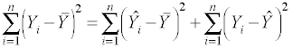
where Y is the response or observed variable,
is the mean and  is the
predicted score. From now on we won't include all of the subscripts since it
will be understood that the summation is over one to n.
is the
predicted score. From now on we won't include all of the subscripts since it
will be understood that the summation is over one to n.
In an intercept only model the predicted score equals the mean, that is,
= . Therefore, we can replace
with in the sums of squares equation, leading to
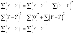
This demonstrates that with an intercept only model there is only residual variability; there is no variability due to the regression model because there are no predictors. Now, let's run an intercept only model and see what it looks like.
regress write

      Source |       SS       df       MS              Number of obs =     200
-------------+------------------------------           F(  0,   199) =    0.00
       Model |           0     0           .           Prob > F      =       .
    Residual |   17878.875   199   89.843593           R-squared     =  0.0000
-------------+------------------------------           Adj R-squared =  0.0000
       Total |   17878.875   199   89.843593           Root MSE      =  9.4786

------------------------------------------------------------------------------
       write |      Coef.   Std. Err.      t    P>|t|     [95% Conf. Interval]
-------------+----------------------------------------------------------------
       _cons |     52.775   .6702372    78.74   0.000     51.45332    54.09668
------------------------------------------------------------------------------
What can we tell from this regression output? First, the constant
is equal to 52.775, which is the mean of the variable write. It is also the
expected or predicted value for every observation. The standard error of the
constant is simply the standard error of variable write. We can manually
compute the standard error from the standard deviation as a check, it is
9.48/sqrt(200) = 0.67. There is no R2 and no overall F-ratio for the model -- both
of which can predicted from working through the partitioning of the sums of
squares. The R2 is equal to SSmodel/SStotal and since
the SSmodel = 0 the
R2 = 0. Technically, the F-ratio doesn't exist at all. Consider the equation,
Since the degrees of freedom for the model are zero (no predictors) and division by zero is undefined so the F-ratio should also be undefined and not zero.
The t-test of the constant tests whether the constant is significantly different from zero. It is also possible to test whether the constant is significantly different from any value, say 50. It is just a matter of subtracting the hypothesized value from the constant and dividing by the standard error of the constant.
This is equivalent to doing a single-sample t-test. Most statistics packages will let you do the test that the constant equals 50, so that you won't have to do the computation by hand.
It is also possible do the above t-test using an intercept only regression model. Lets create a new dependent variable called write50, in which we take the response variable, write, and subtract 50 from each value. We can then run an intercept only model with write50 as the response variable. The value of t given in the output below is the same value that we computed manually above. The constant term, 2.755, in this model is the difference between the overall mean of write and the value 50. This is because we have set up our regression equation to be Y - 50 = a + ε and this leads to E(Y) - 50 = a.
generate write50 = write - 50

regress write50

      Source |       SS       df       MS              Number of obs =     200
-------------+------------------------------           F(  0,   199) =    0.00
       Model |           0     0           .           Prob > F      =       .
    Residual |   17878.875   199   89.843593           R-squared     =  0.0000
-------------+------------------------------           Adj R-squared =  0.0000
       Total |   17878.875   199   89.843593           Root MSE      =  9.4786

------------------------------------------------------------------------------
     write50 |      Coef.   Std. Err.      t    P>|t|     [95% Conf. Interval]
-------------+----------------------------------------------------------------
       _cons |      2.775   .6702372     4.14   0.000     1.453321    4.096679
------------------------------------------------------------------------------
Creating a constantIt is possible for us to create a constant of our own. To do this we make a new variable called one that is equal to the value one. Then, we run a model in which we use one as a predictor. We will have to tell the program we are using not to automatically include a constant in the model. This is the, so called, "no constant" model. The model and output are shown below.
generate one = 1

regress write one, nocons

      Source |       SS       df       MS              Number of obs =     200
-------------+------------------------------           F(  1,   199) = 6200.11
       Model |  557040.125     1  557040.125           Prob > F      =  0.0000
    Residual |   17878.875   199   89.843593           R-squared     =  0.9689
-------------+------------------------------           Adj R-squared =  0.9687
       Total |      574919   200    2874.595           Root MSE      =  9.4786

------------------------------------------------------------------------------
       write |      Coef.   Std. Err.      t    P>|t|     [95% Conf. Interval]
-------------+----------------------------------------------------------------
         one |     52.775   .6702372    78.74   0.000     51.45332    54.09668
------------------------------------------------------------------------------
There are many items that are the same in this model and the intercep-only
model above. The value of the coefficient for the predictor one is the
same as for the constant and has the same standard error and
t-value. But there are also several things that are funny or "wrong" about this
model.There are values for the overall F-ratio and for R2 . Further, the values of these two statistics are wrong. To see why this has happened we need to understand more about the no constant model.
The reason for these differences lies in the fact that the "no constant" model assumes that the mean of the response variable is zero. It will be made clearer when we look once again at the partitioning of the sums of squares substituting zero for the value of the mean.
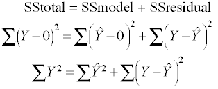
Recall that the predicted score for each observation is the mean of the response variable which is 52.775, thus the sum of squares for the model would be,
 .
.While the sum of squares total is,
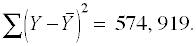 .
.Thus,
and,
Both of which are bogus because the sums of squares for the model are artifically inflated due to using zero instead of the actual mean.
Some statistics packages allow you to run the model with an option to indicate that you have included a constant. With this "has constant" option the program does not compute a constant but uses the constant predictor as the constant for the model. The "has constant" model computes sums of squares and degrees of freedom correctly. These results below look, in fact, exactly like the results in our intercept-only model above.
regress write one, hascons

      Source |       SS       df       MS              Number of obs =     200
-------------+------------------------------           F(  0,   199) =    0.00
       Model |           0     0           .           Prob > F      =       .
    Residual |   17878.875   199   89.843593           R-squared     =  0.0000
-------------+------------------------------           Adj R-squared =  0.0000
       Total |   17878.875   199   89.843593           Root MSE      =  9.4786

------------------------------------------------------------------------------
       write |      Coef.   Std. Err.      t    P>|t|     [95% Conf. Interval]
-------------+----------------------------------------------------------------
         one |     52.775   .6702372    78.74   0.000     51.45332    54.09668
------------------------------------------------------------------------------
With both the "no constant" and the "has constant" approaches you are
not restricted to creating a constant equal to one. You could, for example,
set a constant equal to two, in which case the value of the coefficient would
be half the value of the mean and the standard error is also half as large so
that the t-test is identical to previous models. The output below shows the results
of this model.
generate two = 2

regress write two, hascons

      Source |       SS       df       MS              Number of obs =     200
-------------+------------------------------           F(  0,   199) =    0.00
       Model |           0     0           .           Prob > F      =       .
    Residual |   17878.875   199   89.843593           R-squared     =  0.0000
-------------+------------------------------           Adj R-squared =  0.0000
       Total |   17878.875   199   89.843593           Root MSE      =  9.4786

------------------------------------------------------------------------------
       write |      Coef.   Std. Err.      t    P>|t|     [95% Conf. Interval]
-------------+----------------------------------------------------------------
         two |    26.3875   .3351186    78.74   0.000     25.72666    27.04834
------------------------------------------------------------------------------
Please note, we said you could set the constant equal to two but we are
not sure why anyone would want to do so. Conclusion
What we have established, in this unit, is that the constant in an OLS regression model has something to do with the mean of the response variable. In particular, in intercept only models the constant is equal to the mean of the response variable.