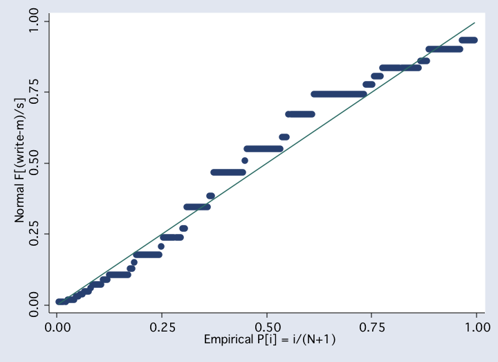
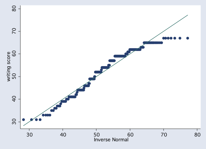
 qnorm write
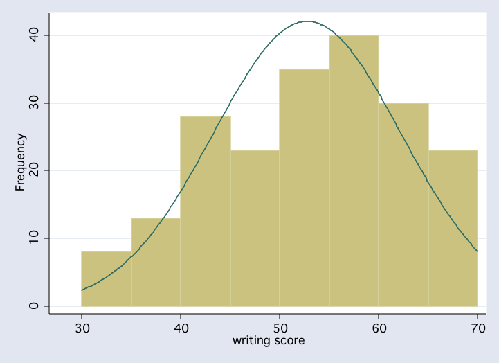
 histogram write, start(30) width(5) normal freq
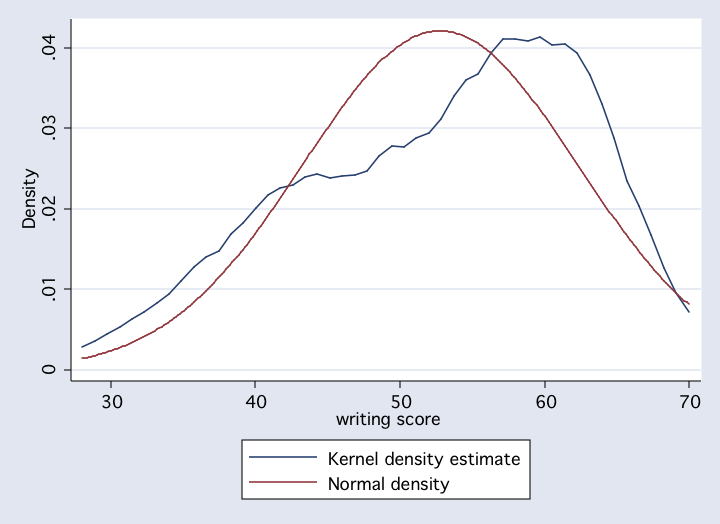
 kdensity write, normal
Displaying Raw Anova Data
Althought it isn't done for every analysis, there will be times that you want to display the raw data for an anova. The tabdisp command allows you to display the anova data in tabular form.
use http://www.philender.com/courses/data/cr4a, clear

sort grp

by grp: generate order = _n  /* number observations within each group */

tabdisp order grp, cellvar(y)

----------------------------------
          |          grp
    order |    1     2     3     4
----------+-----------------------
        1 |    3     4     7     7
        2 |    6     5     8     8
        3 |    3     4     7     9
        4 |    3     3     6     8
        5 |    1     2     5    10
        6 |    2     3     6    10
        7 |    2     4     5     9
        8 |    2     3     6    11
----------------------------------


use http://www.philender.com/courses/data/crf33, clear

sort a b

by a b: generate order = _n  /* number observations within each cell */

tabdisp order b a, cellvar(y)

--------------------------------------------------------------------
          |                         a and b
          | ------- 1 ------    ------- 2 ------    ------- 3 ------
    order |    1     2     3       1     2     3       1     2     3
----------+---------------------------------------------------------
        1 |   37    44    38      34    35    36      21    39    52
        2 |   42    36    28      30    27    45      31    50    53
        3 |   29    27    48      26    40    26      10    34    64
        4 |   33    43    29      39    31    46      20    41    42
        5 |   24    25    47      21    22    27      18    36    49
--------------------------------------------------------------------
General Descriptive and Exploratory Data AnalysisIn general, it is important to look at your data, to try to understand it as best you can. You can use all of the tools in descriptive statistics and exploratory data analysis that were covered in the regression part of the course.
use http://www.philender.com/courses/data/hsb2

describe

Contains data from http://www.gseis.ucla.edu/courses/data/hsb2.dta
  obs:           200                          highschool and beyond (200
                                                cases)
 vars:            11                          21 Jun 2000 08:54
 size:         9,600 (98.9% of memory free)
-------------------------------------------------------------------------------
              storage  display     value
variable name   type   format      label      variable label
-------------------------------------------------------------------------------
id              float  %9.0g
female          float  %9.0g       fl
race            float  %12.0g      rl
ses             float  %9.0g       sl
schtyp          float  %9.0g       scl        type of school
prog            float  %9.0g       sel        type of program
read            float  %9.0g                  reading score
write           float  %9.0g                  writing score
math            float  %9.0g                  math score
science         float  %9.0g                  science score
socst           float  %9.0g                  social studies score
-------------------------------------------------------------------------------

summarize read write math science

    Variable |     Obs        Mean   Std. Dev.       Min        Max
-------------+-----------------------------------------------------
        read |     200       52.23   10.25294         28         76
       write |     200      52.775   9.478586         31         67
        math |     200      52.645   9.368448         33         75
     science |     200       51.85   9.900891         26         74

tab1 female prog

-> tabulation of female

     female |      Freq.     Percent        Cum.
------------+-----------------------------------
       male |         91       45.50       45.50
     female |        109       54.50      100.00
------------+-----------------------------------
      Total |        200      100.00

-> tabulation of prog

    type of |
    program |      Freq.     Percent        Cum.
------------+-----------------------------------
    general |         45       22.50       22.50
   academic |        105       52.50       75.00
   vocation |         50       25.00      100.00
------------+-----------------------------------
      Total |        200      100.00

stem write

Stem-and-leaf plot for write (writing score)

  3* | 1111
  3t | 3333
  3f | 55
  3s | 66777
  3. | 899999
  4* | 0001111111111
  4t | 223
  4f | 4444444444445
  4s | 66666666677
  4. | 99999999999
  5* | 00
  5t | 2222222222222223
  5f | 44444444444444444555
  5s | 777777777777
  5. | 9999999999999999999999999
  6* | 00001111
  6t | 2222222222222222223333
  6f | 5555555555555555
  6s | 7777777

pnorm write


qnorm write


histogram write, start(30) width(5) normal freq


kdensity write, normal
Looking at Data by GroupIn addition to exploratory data analysis and general descriptive statistics you will want to look at data separately for each group in order to check on how well our data meet the assumptions of analysis of variance, in particular, the assumptions of normality and homogeneity of variance (homoscedasticity).
In analysis of variance, we often want to look at the variability and shape of the distribution within each cell of the design. Say that we wanted to look at the anova model for write with female and prog as our categorical variables. There are two levels of female and three levels of prog resulting in a total of six cells. Here are some commands that we can use to look at the data at the marginal and/or cell level.
graph box write, over(female)Graphing Cell Meansgraph box write, over(prog)
graph box write, over(female) over(prog)
tabstat write, stat(n mean sd var) by(prog) Summary for variables: write by categories of: prog (type of program) prog | N mean sd variance ---------+---------------------------------------- general | 45 51.33333 9.397775 88.31818 academic | 105 56.25714 7.943343 63.0967 vocation | 50 46.76 9.318754 86.83918 ---------+---------------------------------------- Total | 200 52.775 9.478586 89.84359 -------------------------------------------------- tabulate female prog, summ(write) Means, Standard Deviations and Frequencies of writing score | type of program female | general academic vocation | Total -----------+---------------------------------+---------- male | 49.142857 54.617021 41.826087 | 50.120879 | 10.364776 8.6566215 8.0037047 | 10.305161 | 21 47 23 | 91 -----------+---------------------------------+---------- female | 53.25 57.586207 50.962963 | 54.990826 | 8.2052475 7.1156721 8.3411929 | 8.1337152 | 24 58 27 | 109 -----------+---------------------------------+---------- Total | 51.333333 56.257143 46.76 | 52.775 | 9.3977754 7.9433433 9.3187544 | 9.478586 | 45 105 50 | 200 /* or you could use */ table female prog, contents(freq mean write sd write) row col -------------------------------------------------- | type of program female | general academic vocation Total ----------+--------------------------------------- male | 21 47 23 91 | 49.14286 54.61702 41.82609 50.12088 | 10.36478 8.656622 8.003705 10.30516 | female | 24 58 27 109 | 53.25 57.58621 50.96296 54.99083 | 8.205248 7.115672 8.341193 8.133716 | Total | 45 105 50 200 | 51.33333 56.25714 46.76 52.775 | 9.397776 7.943343 9.318754 9.478586 -------------------------------------------------- /* or you could use margins */ quietly anova write female##prog margins female#prog, asbalanced Adjusted predictions Number of obs = 200 Expression : Linear prediction, predict() ------------------------------------------------------------------------------ | Delta-method | Margin Std. Err. z P>|z| [95% Conf. Interval] -------------+---------------------------------------------------------------- female#prog | 0 1 | 49.14286 1.803321 27.25 0.000 45.60841 52.6773 0 2 | 54.61702 1.205407 45.31 0.000 52.25447 56.97958 0 3 | 41.82609 1.723133 24.27 0.000 38.44881 45.20337 1 1 | 53.25 1.686852 31.57 0.000 49.94383 56.55617 1 2 | 57.58621 1.085097 53.07 0.000 55.45946 59.71296 1 3 | 50.96296 1.59038 32.04 0.000 47.84588 54.08005 ------------------------------------------------------------------------------ /* or you could use */ sort female prog by female prog: sum(write) _______________________________________________________________________________ -> female = male, prog = general Variable | Obs Mean Std. Dev. Min Max -------------+----------------------------------------------------- write | 21 49.14286 10.36478 31 65 _______________________________________________________________________________ -> female = male, prog = academic Variable | Obs Mean Std. Dev. Min Max -------------+----------------------------------------------------- write | 47 54.61702 8.656621 33 67 _______________________________________________________________________________ -> female = male, prog = vocation Variable | Obs Mean Std. Dev. Min Max -------------+----------------------------------------------------- write | 23 41.82609 8.003705 31 63 _______________________________________________________________________________ -> female = female, prog = general Variable | Obs Mean Std. Dev. Min Max -------------+----------------------------------------------------- write | 24 53.25 8.205248 36 67 _______________________________________________________________________________ -> female = female, prog = academic Variable | Obs Mean Std. Dev. Min Max -------------+----------------------------------------------------- write | 58 57.58621 7.115672 37 67 _______________________________________________________________________________ -> female = female, prog = vocation Variable | Obs Mean Std. Dev. Min Max -------------+----------------------------------------------------- write | 27 50.96296 8.341193 35 67 hist write, by(female prog) normal start(30) width(5) /* stata 8 */ (bin=7, start=30, width=5)
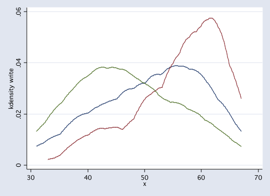
twoway kdensity write, by(prog)
twoway (kdensity write if prog==1)(kdensity write if prog==2)(kdensity write if prog==3), legend(off)
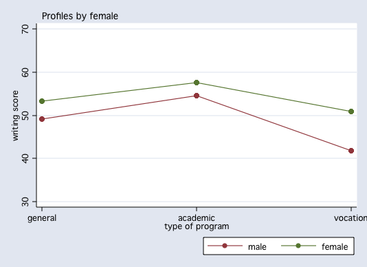
In addition to looking at the data to check on assumptions, it is often useful to graph the cell means as a way to help understand interactions. In this example, we will be using the anovaplot command.
anova write prog female prog#female


                           Number of obs =     200     R-squared     =  0.2590
                           Root MSE      = 8.26386     Adj R-squared =  0.2399

                  Source |  Partial SS    df       MS           F     Prob > F
             ------------+----------------------------------------------------
                   Model |  4630.36091     5  926.072182      13.56     0.0000
                         |
                    prog |  3274.35082     2  1637.17541      23.97     0.0000
                  female |  1261.85329     1  1261.85329      18.48     0.0000
             prog#female |  325.958189     2  162.979094       2.39     0.0946
                         |
                Residual |  13248.5141   194  68.2913097
             ------------+----------------------------------------------------
                   Total |   17878.875   199   89.843593

anovaplot prog female, scatter(msym(none))   /* findit anovaplot */
Linear Statistical Models Course
Phil Ender, 17sep10, 18mar03; 27mar02; 23feb01