
SPF-p.q
Schematic of SPF-2.4 with Example Data
Level S b1
b2 b3 b4
a1 s1
s2
s3
s4
3
6
3
3
4
5
4
3
7
8
7
6
7
8
9
8
a2 s5
s6
s7
s81
2
2
2
2
3
4
35
6
5
610
10
9
11
Or in abbreviated form.
| Level | b1 | b2 | b3 | b4 |
| a1 | S1 n = 4 | S1 n = 4 | S1 n = 4 | S1 n = 4 |
| a2 | S2 n = 4 | S2 n = 4 | S2 n = 4 | S2 n = 4 |
Linear Model
Yijk = μ + αj + πi(j) + βk + αβjk + βπki(j) + εijk
where
μ = overall poulation mean
αj = the effect of treatment level j
πi = the effect of block i
βk = the effect of treatment level k
αβjk = the joint effects of treatment levels j & k
βπki(j) = the effect of treatment level k & block i nested in j of A
εijk = experimental error
Hypotheses
Assumptions
Independence
Normality
Homogeneity of Variance
Independence
Normality
Compound Symmetry in the Variance-Covariance Matrix
No nonadditivity
ANOVA Summary Table
| Source | SS | df | MS | F | p-value | Error | |
| Between Blocks | |||||||
| 1 | A | 3.125 | 1 | 3.125 | 2.00 | .2070 | [2] |
| 2 | Blks(A) | 9.375 | 6 | 1.562 | |||
| Within Blocks | |||||||
| 3 | B | 194.500 | 3 | 64.833 | 127.88 | .0000 | [5] |
| 4 | A*B | 19.375 | 3 | 6.458 | 12.74 | .0001 | [5] |
| 5 | B*Blks(A) | 9.125 | 18 | 0.507 | |||
| Total | 235.500 | 31 | |||||
Expected Mean Squares
E(MS a)          = σ2ε + qσ2π + nqσ2α
E(MS blks(a))    = σ2ε + qσ2π
E(MS b)          = σ2ε + σ2βπ + npσ2β
E(MS a#b)        = σ2ε + σ2βπ + nσ2αβ
E(MS b#blks(a))  = σ2ε + σ2βπ
Strength of Association
F-ratio is not significant, do not compute omega2 for A.
Using Stata
input y a b s x1 x2 x3 x4 s1 s2 s3 s4 s5 s6
3 1 1 1 1 1 1 1 1 1 1 0 0 0
6 1 1 2 1 1 1 1 -1 1 1 0 0 0
3 1 1 3 1 1 1 1 0 -2 1 0 0 0
3 1 1 4 1 1 1 1 0 0 -3 0 0 0
1 2 1 5 -1 1 1 1 0 0 0 1 1 1
2 2 1 6 -1 1 1 1 0 0 0 -1 1 1
2 2 1 7 -1 1 1 1 0 0 0 0 -2 1
2 2 1 8 -1 1 1 1 0 0 0 0 0 -3
4 1 2 1 1 -1 1 1 1 1 1 0 0 0
5 1 2 2 1 -1 1 1 -1 1 1 0 0 0
4 1 2 3 1 -1 1 1 0 -2 1 0 0 0
3 1 2 4 1 -1 1 1 0 0 -3 0 0 0
2 2 2 5 -1 -1 1 1 0 0 0 1 1 1
3 2 2 6 -1 -1 1 1 0 0 0 -1 1 1
4 2 2 7 -1 -1 1 1 0 0 0 0 -2 1
3 2 2 8 -1 -1 1 1 0 0 0 0 0 -3
7 1 3 1 1 0 -2 1 1 1 1 0 0 0
8 1 3 2 1 0 -2 1 -1 1 1 0 0 0
7 1 3 3 1 0 -2 1 0 -2 1 0 0 0
6 1 3 4 1 0 -2 1 0 0 -3 0 0 0
5 2 3 5 -1 0 -2 1 0 0 0 1 1 1
6 2 3 6 -1 0 -2 1 0 0 0 -1 1 1
5 2 3 7 -1 0 -2 1 0 0 0 0 -2 1
6 2 3 8 -1 0 -2 1 0 0 0 0 0 -3
7 1 4 1 1 0 0 -3 1 1 1 0 0 0
8 1 4 2 1 0 0 -3 -1 1 1 0 0 0
9 1 4 3 1 0 0 -3 0 -2 1 0 0 0
8 1 4 4 1 0 0 -3 0 0 -3 0 0 0
10 2 4 5 -1 0 0 -3 0 0 0 1 1 1
10 2 4 6 -1 0 0 -3 0 0 0 -1 1 1
9 2 4 7 -1 0 0 -3 0 0 0 0 -2 1
11 2 4 8 -1 0 0 -3 0 0 0 0 0 -3
end
tabulate a, summ(y)
| Summary of y
a | Mean Std. Dev. Freq.
------------+------------------------------------
1 | 5.6875 2.120338 16
2 | 5.0625 3.3159966 16
------------+------------------------------------
Total | 5.375 2.7562246 32
tabulate b, summ(y)
| Summary of y
b | Mean Std. Dev. Freq.
------------+------------------------------------
1 | 2.75 1.4880476 8
2 | 3.5 .9258201 8
3 | 6.25 1.0350983 8
4 | 9 1.3093073 8
------------+------------------------------------
Total | 5.375 2.7562246 32
table a, cont(freq mean y sd y) by(b)
----------+-----------------------------------
b and a | Freq. mean(y) sd(y)
----------+-----------------------------------
1 |
1 | 4 3.75 1.5
2 | 4 1.75 .5
----------+-----------------------------------
2 |
1 | 4 4 .8164966
2 | 4 3 .8164966
----------+-----------------------------------
3 |
1 | 4 7 .8164966
2 | 4 5.5 .5773503
----------+-----------------------------------
4 |
1 | 4 8 .8164966
2 | 4 10 .8164966
----------+-----------------------------------
histogram y, by(a) normal
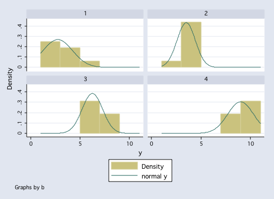
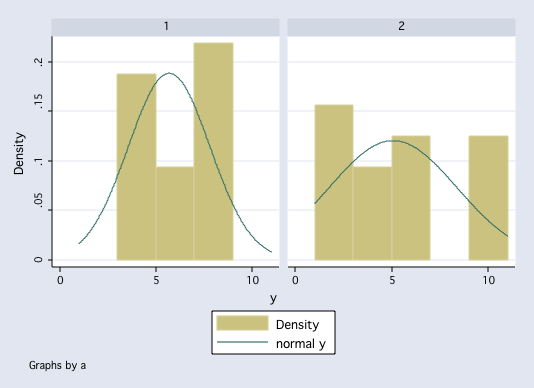 histogram y, by(b) normal
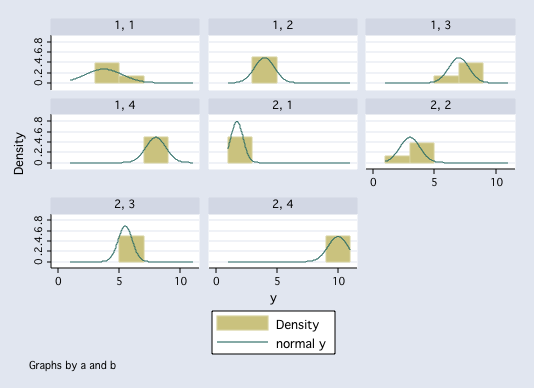
 histogram y, by(a b) normal
 anova y a / s|a b a#b / , repeated(b)
Number of obs = 32 R-squared = 0.9613
Root MSE = .712 Adj R-squared = 0.9333
Source | Partial SS df MS F Prob > F
-----------+----------------------------------------------------
Model | 226.375 13 17.4134615 34.35 0.0000
|
a | 3.125 1 3.125 2.00 0.2070
s|a | 9.375 6 1.5625
-----------+----------------------------------------------------
b | 194.5 3 64.8333333 127.89 0.0000
a#b | 19.375 3 6.45833333 12.74 0.0001
|
Residual | 9.125 18 .506944444
-----------+----------------------------------------------------
Total | 235.5 31 7.59677419
Between-subjects error term: s|a
Levels: 8 (6 df)
Lowest b.s.e. variable: s
Covariance pooled over: a (for repeated variable)
Repeated variable: b
Huynh-Feldt epsilon = 0.9432
Greenhouse-Geisser epsilon = 0.5841
Box's conservative epsilon = 0.3333
------------ Prob > F ------------
Source | df F Regular H-F G-G Box
-----------+----------------------------------------------------
b | 3 127.89 0.0000 0.0000 0.0000 0.0000
a#b | 3 12.74 0.0001 0.0002 0.0019 0.0118
Residual | 18
----------------------------------------------------------------
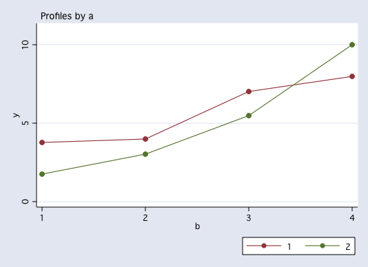
quietly anova y a b a#b /* needed to obtain graphs */
anovaplot b a, scatter(msym(none))
anova y a / s|a b a#b / , repeated(b)
Number of obs = 32 R-squared = 0.9613
Root MSE = .712 Adj R-squared = 0.9333
Source | Partial SS df MS F Prob > F
-----------+----------------------------------------------------
Model | 226.375 13 17.4134615 34.35 0.0000
|
a | 3.125 1 3.125 2.00 0.2070
s|a | 9.375 6 1.5625
-----------+----------------------------------------------------
b | 194.5 3 64.8333333 127.89 0.0000
a#b | 19.375 3 6.45833333 12.74 0.0001
|
Residual | 9.125 18 .506944444
-----------+----------------------------------------------------
Total | 235.5 31 7.59677419
Between-subjects error term: s|a
Levels: 8 (6 df)
Lowest b.s.e. variable: s
Covariance pooled over: a (for repeated variable)
Repeated variable: b
Huynh-Feldt epsilon = 0.9432
Greenhouse-Geisser epsilon = 0.5841
Box's conservative epsilon = 0.3333
------------ Prob > F ------------
Source | df F Regular H-F G-G Box
-----------+----------------------------------------------------
b | 3 127.89 0.0000 0.0000 0.0000 0.0000
a#b | 3 12.74 0.0001 0.0002 0.0019 0.0118
Residual | 18
----------------------------------------------------------------
quietly anova y a b a#b /* needed to obtain graphs */
anovaplot b a, scatter(msym(none))
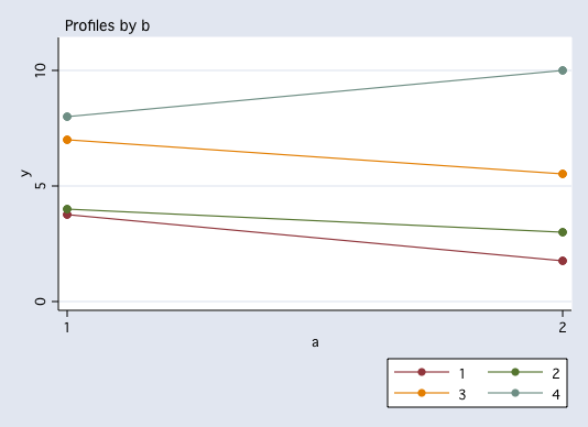
 anovaplot a b, scatter(msym(none))
Using Stata: Regression with Orthogonal Coding
generate x5=x1*x2
generate x6=x1*x3
generate x7=x1*x4

regress y x1 x2 x3 x4 x5 x6 x7 s1 s2 s3 s4 s5 s6


      Source |       SS       df       MS              Number of obs =      32
-------------+------------------------------           F( 13,    18) =   34.35
       Model |     226.375    13  17.4134615           Prob > F      =  0.0000
    Residual |       9.125    18  .506944444           R-squared     =  0.9613
-------------+------------------------------           Adj R-squared =  0.9333
       Total |       235.5    31  7.59677419           Root MSE      =    .712

------------------------------------------------------------------------------
           y |      Coef.   Std. Err.      t    P>|t|     [95% Conf. Interval]
-------------+----------------------------------------------------------------
          x1 |      .3125   .1258651     2.48   0.023     .0480673    .5769327
          x2 |      -.375   .1780001    -2.11   0.049    -.7489643   -.0010357
          x3 |  -1.041667   .1027684   -10.14   0.000    -1.257575   -.8257583
          x4 |  -1.208333   .0726682   -16.63   0.000    -1.361004   -1.055663
          x5 |        .25   .1780001     1.40   0.177    -.1239643    .6239643
          x6 |          0   .1027684     0.00   1.000    -.2159084    .2159084
          x7 |      .4375   .0726682     6.02   0.000     .2848297    .5901703
          s1 |       -.75   .2517301    -2.98   0.008    -1.278865   -.2211346
          s2 |   .0833333   .1453365     0.57   0.573    -.2220072    .3886739
          s3 |   .2291667   .1027684     2.23   0.039     .0132583     .445075
          s4 |      -.375   .2517301    -1.49   0.154    -.9038654    .1538654
          s5 |  -.0416667   .1453365    -0.29   0.778    -.3470072    .2636739
          s6 |  -.1458333   .1027684    -1.42   0.173    -.3617417     .070075
       _cons |      5.375   .1258651    42.70   0.000     5.110567    5.639433
------------------------------------------------------------------------------

test2 x1 / s1 s2 s3 s4 s5 s6

Testing: x1
Error term: s1 s2 s3 s4 s5 s6

     F(  1,   6)  =     2.00
         Prob > F =     0.2070

test x2 x3 x4

 ( 1)  x2 = 0
 ( 2)  x3 = 0
 ( 3)  x4 = 0

       F(  3,    18) =  127.89
            Prob > F =    0.0000

test x5 x6 x7

 ( 1)  x5 = 0
 ( 2)  x6 = 0
 ( 3)  x7 = 0

       F(  3,    18) =   12.74
            Prob > F =    0.0001
Using Stata: Data in Wide Forminput s a y1 y2 y3 y4 1 1 3 4 7 7 2 1 6 5 8 8 3 1 3 4 7 9 4 1 3 3 6 8 5 2 1 2 5 10 6 2 2 3 6 10 7 2 2 4 5 9 8 2 2 3 6 11
The Multivariate Approach
Using the manova command.
manova y1 y2 y3 y4 = a

                           Number of obs =       8

                           W = Wilks' lambda      L = Lawley-Hotelling trace
                           P = Pillai's trace     R = Roy's largest root

                  Source |  Statistic     df   F(df1,    df2) =   F   Prob>F
              -----------+--------------------------------------------------
                       a | W   0.1374      1     4.0     3.0     4.71 0.1169 e
                         | P   0.8626            4.0     3.0     4.71 0.1169 e
                         | L   6.2764            4.0     3.0     4.71 0.1169 e
                         | R   6.2764            4.0     3.0     4.71 0.1169 e
                         |--------------------------------------------------
                Residual |                 6
              -----------+--------------------------------------------------
                   Total |                 7
              --------------------------------------------------------------
                           e = exact, a = approximate, u = upper bound on

mat ymat = (1,0,0,-1\0,1,0,-1\0,0,1,-1)

mat list ymat

ymat[3,4]
    c1  c2  c3  c4
r1   1   0   0  -1
r2   0   1   0  -1
r3   0   0   1  -1

/* test of the y#a interaction */

manovatest a, ytransform(ymat)

 Transformations of the dependent variables
 (1)    y1 - y4
 (2)    y2 - y4
 (3)    y3 - y4

                           W = Wilks' lambda      L = Lawley-Hotelling trace
                           P = Pillai's trace     R = Roy's largest root

                  Source |  Statistic     df   F(df1,    df2) =   F   Prob>F
              -----------+--------------------------------------------------
                       a | W   0.1443      1     3.0     4.0     7.91 0.0371 e
                         | P   0.8557            3.0     4.0     7.91 0.0371 e
                         | L   5.9296            3.0     4.0     7.91 0.0371 e
                         | R   5.9296            3.0     4.0     7.91 0.0371 e
                         |--------------------------------------------------
                Residual |                 6
              --------------------------------------------------------------
                           e = exact, a = approximate, u = upper bound on F

/* test of y */

mat xmat = (1, .5, .5)

mat list xmat

xmat[1,3]
    c1  c2  c3
r1   1  .5  .5

manovatest, test(xmat) ytransform(ymat)

 Transformations of the dependent variables
 (1)    y1 - y4
 (2)    y2 - y4
 (3)    y3 - y4

 Test constraint
 (1)    _cons + .5 a[1] + .5 a[2] = 0

                           W = Wilks' lambda      L = Lawley-Hotelling trace
                           P = Pillai's trace     R = Roy's largest root

                  Source |  Statistic     df   F(df1,    df2) =   F   Prob>F
              -----------+--------------------------------------------------
              manovatest | W   0.0275      1     3.0     4.0    47.19 0.0014 e
                         | P   0.9725            3.0     4.0    47.19 0.0014 e
                         | L  35.3944            3.0     4.0    47.19 0.0014 e
                         | R  35.3944            3.0     4.0    47.19 0.0014 e
                         |--------------------------------------------------
                Residual |                 6
              -------------------------------------------------------------
Wide to Long
reshape long y, i(s) j(b)
(note:  j = 1 2 3 4)

Data                               wide   ->   long
-----------------------------------------------------------------------------
Number of obs.                        8   ->      32
Number of variables                   6   ->       4
j variable (4 values)                     ->   b
xij variables:
                           y1 y2 ... y4   ->   y
-----------------------------------------------------------------------------

describe

Contains data
  obs:            32
 vars:             4
 size:           544 (96.8% of memory free)
-------------------------------------------------------------------------------
   1. s         float  %9.0g
   2. b         byte   %9.0g
   3. a         float  %9.0g
   4. y         float  %9.0g
-------------------------------------------------------------------------------
Sorted by:  s  b
     Note:  dataset has changed since last saved

tab1 a b s

-> tabulation of a

          a |      Freq.     Percent        Cum.
------------+-----------------------------------
          1 |         16       50.00       50.00
          2 |         16       50.00      100.00
------------+-----------------------------------
      Total |         32      100.00

-> tabulation of b

          b |      Freq.     Percent        Cum.
------------+-----------------------------------
          1 |          8       25.00       25.00
          2 |          8       25.00       50.00
          3 |          8       25.00       75.00
          4 |          8       25.00      100.00
------------+-----------------------------------
      Total |         32      100.00

-> tabulation of s

          s |      Freq.     Percent        Cum.
------------+-----------------------------------
          1 |          4       12.50       12.50
          2 |          4       12.50       25.00
          3 |          4       12.50       37.50
          4 |          4       12.50       50.00
          5 |          4       12.50       62.50
          6 |          4       12.50       75.00
          7 |          4       12.50       87.50
          8 |          4       12.50      100.00
------------+-----------------------------------
      Total |         32      100.00
The Univariate Anova Approach
The univariate anova approach would uses the anova command like this.
anova y a / s|a b a#b /, repeat(b)

                           Number of obs =      32     R-squared     =  0.9613
                           Root MSE      =    .712     Adj R-squared =  0.9333

                  Source |  Partial SS    df       MS           F     Prob > F
              -----------+----------------------------------------------------
                   Model |     226.375    13  17.4134615      34.35     0.0000
                         |
                       a |       3.125     1       3.125       2.00     0.2070
                     s|a |       9.375     6      1.5625
              -----------+----------------------------------------------------
                       b |       194.5     3  64.8333333     127.89     0.0000
                     a#b |      19.375     3  6.45833333      12.74     0.0001
                         |
                Residual |       9.125    18  .506944444
              -----------+----------------------------------------------------
                   Total |       235.5    31  7.59677419


Between-subjects error term:  s|a
                     Levels:  8         (6 df)
     Lowest b.s.e. variable:  s
     Covariance pooled over:  a         (for repeated variable)

Repeated variable: b
                                          Huynh-Feldt epsilon        =  0.9432
                                          Greenhouse-Geisser epsilon =  0.5841
                                          Box's conservative epsilon =  0.3333

                                            ------------ Prob > F ------------
                  Source |     df      F    Regular    H-F      G-G      Box
              -----------+----------------------------------------------------
                       b |      3   127.89   0.0000   0.0000   0.0000   0.0000
                     a#b |      3    12.74   0.0001   0.0002   0.0019   0.0118
                Residual |     18
              ----------------------------------------------------------------
Generalized Expected Mean Squares with Sampling Fractions
Sampling Fractions
When A is fixed P' = 0, when A is random P' = 1
When B is fixed Q' = 0, when B is random Q' = 1
When Blocks are fixed N' = 0, when Blocks are random N' = 1
Where P' is a short way of writing 1 - p/P. p/P is the sampling fraction.
P' = 1 - p/P
Q' = 1 - q/Q
N' = 1 - n/N
The Variance-Covariance Matrices
Computing the Variance-Covariance Matrices from Wide Data
input s a y1 y2 y3 y4
1 1 3 4 7  7
2 1 6 5 8  8
3 1 3 4 7  9
4 1 3 3 6  8
5 2 1 2 5 10
6 2 2 3 6 10
7 2 2 4 5  9
8 2 2 3 6 11
end

corr y1 y2 y3 y4 if a==1, cov
(obs=4)

         |       y1       y2       y3       y4
---------+------------------------------------
      y1 |     2.25
      y2 |        1  .666667
      y3 |        1  .666667  .666667
      y4 |        0        0        0  .666667

corr y1 y2 y3 y4 if a==2, cov
(obs=4)

         |       y1       y2       y3       y4
---------+------------------------------------
      y1 |      .25
      y2 |  .333333  .666667
      y3 |  .166667        0  .333333
      y4 |        0 -.333333  .333333  .666667
Pooling the Variance-Covariance Matrices
      b1     b2     b3     b4
b1  1.2500  .6667  .5834      0
b2   .6667  .6667  .3334 -.1667
b3   .5834  .3334  .5000  .1667
b4       0 -.1667  .1667  .6667
Obtaining the Pooled Variance-Covariance Matrice in Stata
anova y a / s|a b a#b /, repeated(b)

[output omitted]

mat lis e(Srep)

symmetric e(Srep)[4,4]
            c1          c2          c3          c4
r1        1.25
r2   .66666667   .66666667
r3   .58333333   .33333333          .5
r4           0  -.16666667   .16666667   .66666667
Conservative F-ratios
Here are the results from the anova command displaying the conventional and conservative p-values.
                                    Huynh-Feldt epsilon        =  0.9432
                                    Greenhouse-Geisser epsilon =  0.5841
                                    Box's conservative epsilon =  0.3333

                                      ------------ Prob > F ------------
            Source |     df      F    Regular    H-F      G-G      Box
        -----------+----------------------------------------------------
                 b |      3   127.89   0.0000   0.0000   0.0000   0.0000
               a*b |      3    12.74   0.0001   0.0002   0.0019   0.0118
          Residual |     18
        -----------+----------------------------------------------------
Tests of Simple Main Effects
ANOVA Summary Table
| Source | SS | df | MS | F | Error Term | |
| Between Blocks | ||||||
| 1 | A at b1 | 8.000 | 1 | 8.000 | 10.38 | [5] |
| 2 | A at b2 | 2.000 | 1 | 2.000 | 2.59 | [5] |
| 3 | A at b3 | 4.500 | 1 | 4.500 | 5.84 | [5] |
| 4 | A at b4 | 8.000 | 1 | 8.000 | 10.38 | [5] |
| 5 | Within cell | 18.500 | 24 | .771 | ||
| Within Blocks | ||||||
| 6 | B at a1 | 54.687 | 3 | 18.229 | 35.95 | [9] |
| 7 | B at a2 | 159.187 | 3 | 53.062 | 104.66 | [9] |
| 8 | A*B | 19.375 | 3 | 6.458 | 12.74 | [9] |
| 9 | B*Blks(A) | 9.125 | 18 | 0.507 | ||
| Total | 235.500 | 31 | ||||
Using Stata
anova y a / s|a b a#b /, repeated(b)


                           Number of obs =      32     R-squared     =  0.9613
                           Root MSE      =    .712     Adj R-squared =  0.9333

                  Source |  Partial SS    df       MS           F     Prob > F
              -----------+----------------------------------------------------
                   Model |     226.375    13  17.4134615      34.35     0.0000
                         |
                       a |       3.125     1       3.125       2.00     0.2070
                     s|a |       9.375     6      1.5625
              -----------+----------------------------------------------------
                       b |      194.50     3  64.8333333     127.89     0.0000
                     a*b |      19.375     3  6.45833333      12.74     0.0001
                         |
                Residual |       9.125    18  .506944444
              -----------+----------------------------------------------------
                   Total |      235.50    31  7.59677419


Between-subjects error term:  s|a
                     Levels:  8         (6 df)
     Lowest b.s.e. variable:  s
     Covariance pooled over:  a         (for repeated variable)

Repeated variable: b
                                          Huynh-Feldt epsilon        =  0.9432
                                          Greenhouse-Geisser epsilon =  0.5841
                                          Box's conservative epsilon =  0.3333

                                            ------------ Prob > F ------------
                  Source |     df      F    Regular    H-F      G-G      Box
              -----------+----------------------------------------------------
                       b |      3   127.89   0.0000   0.0000   0.0000   0.0000
                     a*b |      3    12.74   0.0001   0.0002   0.0019   0.0118
                Residual |     18
              -----------+----------------------------------------------------


sme a b, sse(18.5) dfe(24)    /* combines df & ss for s|a and residual */

Test of a at b(1): F(1/24)  = 10.378378
Test of a at b(2): F(1/24)  = 2.5945946
Test of a at b(3): F(1/24)  = 5.8378378
Test of a at b(4): F(1/24)  = 10.378378


Critical value of F for alpha = .05 using ...
--------------------------------------------------
Dunn's procedure              = 5.7165623
Marascuilo & Levin            = 6.623745
per family error rate         = 7.291317
simultaneous test procedure   = 20.978425

sme b a

Test of b at a(1): F(3/18)  = 35.958904
Test of b at a(2): F(3/18)  = 104.67123


Critical value of F for alpha = .05 using ...
--------------------------------------------------
Dunn's procedure              = 3.9538741
Marascuilo & Levin            = 4.4443607
per family error rate         = 3.9538741
simultaneous test procedure   = 7.3122283

tkcomp b if a==1

Tukey-Kramer pairwise comparisons for variable b
studentized range critical value(.05, 4, 18) = 3.9970087

                                      mean
grp vs grp       group means          dif     TK-test
-------------------------------------------------------
  1 vs   2     3.7500     4.0000      0.2500   0.7022
  1 vs   3     3.7500     7.0000      3.2500   9.1292*
  1 vs   4     3.7500     8.0000      4.2500  11.9382*
  2 vs   3     4.0000     7.0000      3.0000   8.4270*
  2 vs   4     4.0000     8.0000      4.0000  11.2360*
  3 vs   4     7.0000     8.0000      1.0000   2.8090

tkcomp b if a==2

Tukey-Kramer pairwise comparisons for variable b
studentized range critical value(.05, 4, 18) = 3.9970087

                                      mean
grp vs grp       group means          dif     TK-test
-------------------------------------------------------
  1 vs   2     1.7500     3.0000      1.2500   3.5112
  1 vs   3     1.7500     5.5000      3.7500  10.5337*
  1 vs   4     1.7500    10.0000      8.2500  23.1741*
  2 vs   3     3.0000     5.5000      2.5000   7.0225*
  2 vs   4     3.0000    10.0000      7.0000  19.6629*
  3 vs   4     5.5000    10.0000      4.5000  12.6404*
Linear Mixed Models Approach
xtmixed y a##b || s:, var

Performing EM optimization:

Performing gradient-based optimization:

Iteration 0:   log restricted-likelihood = -34.824381
Iteration 1:   log restricted-likelihood = -34.824379

Computing standard errors:

Mixed-effects REML regression                   Number of obs      =        32
Group variable: s                               Number of groups   =         8

                                                Obs per group: min =         4
                                                               avg =       4.0
                                                               max =         4


                                                Wald chi2(7)       =    423.89
Log restricted-likelihood = -34.824379          Prob > chi2        =    0.0000

------------------------------------------------------------------------------
           y |      Coef.   Std. Err.      z    P>|z|     [95% Conf. Interval]
-------------+----------------------------------------------------------------
         2.a |         -2   .6208193    -3.22   0.001    -3.216783   -.7832165
             |
           b |
          2  |        .25   .5034603     0.50   0.619     -.736764    1.236764
          3  |       3.25   .5034603     6.46   0.000     2.263236    4.236764
          4  |       4.25   .5034603     8.44   0.000     3.263236    5.236764
             |
         a#b |
        2 2  |          1   .7120004     1.40   0.160    -.3954951    2.395495
        2 3  |         .5   .7120004     0.70   0.483    -.8954951    1.895495
        2 4  |          4   .7120004     5.62   0.000     2.604505    5.395495
             |
       _cons |       3.75   .4389855     8.54   0.000     2.889604    4.610396
------------------------------------------------------------------------------

------------------------------------------------------------------------------
  Random-effects Parameters  |   Estimate   Std. Err.     [95% Conf. Interval]
-----------------------------+------------------------------------------------
s: Identity                  |
                  var(_cons) |   .2638887   .2294499      .0480071    1.450562
-----------------------------+------------------------------------------------
               var(Residual) |   .5069445   .1689815      .2637707    .9743036
------------------------------------------------------------------------------
LR test vs. linear regression: chibar2(01) =     3.30 Prob >= chibar2 = 0.0346

anovalator a b, main 2way fratio

anovalator main-effect for a
chi2(1) = 2.000001   p-value = .1572991
scaled as F-ratio = 2.000001

anovalator main-effect for b
chi2(3) = 383.67117   p-value = 7.619e-83
scaled as F-ratio = 127.89039

anovalator two-way interaction for a#b
chi2(3) = 38.219172   p-value = 2.540e-08
scaled as F-ratio = 12.739724

anovalator a b, simple fratio

anovalator test of simple main effects for a at(b=1)
chi2(1) = 10.37838   p-value = .001275
scaled as F-ratio = 10.37838

anovalator test of simple main effects for a at(b=2)
chi2(1) = 2.594595   p-value = .10722884
scaled as F-ratio = 2.594595

anovalator test of simple main effects for a at(b=3)
chi2(1) = 5.8378388   p-value = .01568508
scaled as F-ratio = 5.8378388

anovalator test of simple main effects for a at(b=4)
chi2(1) = 10.37838   p-value = .001275
scaled as F-ratio = 10.37838

anovalator b a, simple fratio

anovalator test of simple main effects for b at(a=1)
chi2(3) = 107.87669   p-value = 3.142e-23
scaled as F-ratio = 35.958898

anovalator test of simple main effects for b at(a=2)
chi2(3) = 314.01365   p-value = 9.217e-68
scaled as F-ratio = 104.67122

anovalator b , pair at(a=1) quietly

anovalator pairwise comparisons for b at(a=1)

Comparison          Coef.   Std. Err.      z    P>|z|     [95% Conf. Interval]
1 vs 2               -.25     .50346    -.497   0.619    -1.236782    .7367822
1 vs 3              -3.25     .50346    -6.46   0.000    -4.236782   -2.263218
1 vs 4              -4.25     .50346    -8.44   0.000    -5.236782   -3.263218
2 vs 3                 -3     .50346    -5.96   0.000    -3.986782   -2.013218
2 vs 4                 -4     .50346    -7.95   0.000    -4.986782   -3.013218
3 vs 4                 -1     .50346    -1.99   0.047    -1.986782  -.01321783

anovalator b , pair at(a=2) quietly

anovalator pairwise comparisons for b at(a=2)

Comparison          Coef.   Std. Err.      z    P>|z|     [95% Conf. Interval]
1 vs 2              -1.25     .50346    -2.48   0.013    -2.236782   -.2632178
1 vs 3              -3.75     .50346    -7.45   0.000    -4.736782   -2.763218
1 vs 4              -8.25     .50346    -16.4   0.000    -9.236782   -7.263218
2 vs 3               -2.5     .50346    -4.97   0.000    -3.486782   -1.513218
2 vs 4                 -7     .50346    -13.9   0.000    -7.986782   -6.013218
3 vs 4               -4.5     .50346    -8.94   0.000    -5.486782   -3.513218
Linear Statistical Models Course
Phil Ender, 17sep10, 9may06, 25apr06, 5may00, 12Feb98