Power

Power & Sample Size

Linear Statistical Models

A General Statement

A bigger sample is usually better.

Samples can be too big

inefficient
trivial differences show up as significant

Generally, you should try to collect the largest sample size that you can given the resources that you have.

Power

The ability to detect true differences when they exist.

Power is the probability of rejecting the null hypothesis when it is false.

β the probability failing to reject H₀ when it is false.

Therefore, Power = 1 - β.

Power of at least .80 is considered acceptable.

Experimental Decision Table

Truth

Experimenter's
Decision H₀ is true H₀ is false

Fail to reject H₀ Correct Decision
1 - α Type II Error
β

Reject H₀ Type I Error
α Correct Decision
1 - β
Power

Factors that Effect Power

Sample size

Treatment effect size

Alpha level

Error variance

Effect Size

The effect size coefficient, f, expresses the differences among the group means in terms of standard units.

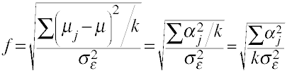
f = .10 -- small effect size
f = .25 -- medium effectg size
f = .40 -- large effect size

An estimate of the effect size, f, can be obtained using ω²

The effectsize command also produces an estimate of effect size using the ω² fomula above. Here are two examples.

use http://www.philender.com/courses/data/cr4new, clear

anova y a

                           Number of obs =      32     R-squared     =  0.4455
                           Root MSE      =   1.476     Adj R-squared =  0.3860

                  Source |  Partial SS    df       MS           F     Prob > F
              -----------+----------------------------------------------------
                   Model |       49.00     3  16.3333333       7.50     0.0008
                         |
                       a |       49.00     3  16.3333333       7.50     0.0008
                         |
                Residual |       61.00    28  2.17857143   
              -----------+----------------------------------------------------
                   Total |      110.00    31   3.5483871  

effectsize a

anova effect size for a with dep var = y

total variance accounted for
omega2         = .37854187
eta2           = .44545455
Cohen's f      = .78046067

partial variance accounted for
partial omega2 = .37854187
partial eta2   = .44545455

 
use http://www.philender.com/courses/data/hsb2

anova write prog

                           Number of obs =     200     R-squared     =  0.1776
                           Root MSE      = 8.63918     Adj R-squared =  0.1693

                  Source |  Partial SS    df       MS           F     Prob > F
              -----------+----------------------------------------------------
                   Model |  3175.69786     2  1587.84893      21.27     0.0000
                         |
                    prog |  3175.69786     2  1587.84893      21.27     0.0000
                         |
                Residual |  14703.1771   197   74.635417   
              -----------+----------------------------------------------------
                   Total |   17878.875   199   89.843593   

effectsize prog

anova effect size for prog with dep var = write

total variance accounted for
omega2         = .16857021
eta2           = .17762291
Cohen's f      = .45027478

partial variance accounted for
partial omega2 = .16857021
partial eta2   = .17762291

Practicalities

Prior to collecting and analyzing data the sizes of treatment effects and error variance are usually unknown.

These values can be estimated from sample data or pilot studies.

One of the challenges of research is to design an experiment that (1) has adequate power to detect meaningful or practical differences, (2) uses minimum resources, n, (3) provides adequate protection against making a type I error, and (4) minimizes the effects of extraneous variables (Kirk, 1995).

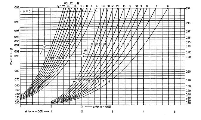
Using Pearson-Hartley Power Curves

alpha - sets of curves for α = .05 and α = .01.
power - enter from the left edge.
ν₁ - df for treatment levels.
φ - ratio of treatment effect to error in terms of number of standard errors.
(f, above, is related to φ by the formula φ = f*sqrt(n) = .7805*sqrt(8) = 2.2 )
ν₂ - df for error (to be estimated from the curves and divided equally among the cells).

Example

Example 1 2

alpha .01 .05
power .80 .80
ν₁ 3 3
φ 2.2 2.2
Read ν₂ 30 7
n per cell* 8 3

To nearest integer per cell.

Power Curve for ν₁ = 3

Using Monte Carlo Simulation

Next, we will do a Monte Carlo power simulation using the simpower command from ATS. Here is how to get the program.

net from http://www.ats.ucla.edu/stat/stata/ado/analysis/
net install simpower

Let's try simulating a three group anova.

simpower, groups(3) n(5 5 5) mu(10 12 14) s(3 3 3)

Sample Sizes, Means and Standard Deviations
-------------------------------------------
N1 = 5        MU1 = 10         S1 = 3
N2 = 5        MU2 = 12         S2 = 3
N3 = 5        MU3 = 14         S3 = 3

 1000 simulated ANOVA F tests
------------------------------
 Alpha   Simulated 
 Level     Power
------------------------------
 0.1000   0.5260       
 0.0750   0.4680       
 0.0500   0.3820       
 0.0250   0.2600       
 0.0100   0.1440       

simpower, groups(3) n(10 10 10) mu(10 12 14) s(3 3 3)

Sample Sizes, Means and Standard Deviations
-------------------------------------------
N1 = 10       MU1 = 10         S1 = 3
N2 = 10       MU2 = 12         S2 = 3
N3 = 10       MU3 = 14         S3 = 3

 1000 simulated ANOVA F tests
------------------------------
 Alpha   Simulated 
 Level     Power
------------------------------
 0.1000   0.8330       
 0.0750   0.7800       
 0.0500   0.7110       
 0.0250   0.5900       
 0.0100   0.4440       

simpower, groups(3) n(15 15 15) mu(10 12 14) s(3 3 3)

Sample Sizes, Means and Standard Deviations
-------------------------------------------
N1 = 15       MU1 = 10         S1 = 3
N2 = 15       MU2 = 12         S2 = 3
N3 = 15       MU3 = 14         S3 = 3

 1000 simulated ANOVA F tests
------------------------------
 Alpha   Simulated 
 Level     Power
------------------------------
 0.1000   0.9400       
 0.0750   0.9280       
 0.0500   0.9050       
 0.0250   0.8350       
 0.0100   0.7160

Next, we will use simpower beginning with a real anova.

use http://www.gseis.ucla.edu/courses/data/crf33

anova y b

                           Number of obs =      45     R-squared     =  0.2957
                           Root MSE      = 9.35626     Adj R-squared =  0.2621

                  Source |  Partial SS    df       MS           F     Prob > F
              -----------+----------------------------------------------------
                   Model |  1543.33333     2  771.666667       8.82     0.0006
                         |
                       b |  1543.33333     2  771.666667       8.82     0.0006
                         |
                Residual |  3676.66667    42  87.5396825   
              -----------+----------------------------------------------------
                   Total |     5220.00    44  118.636364   

simpower y b

Sample Sizes, Means and Standard Deviations
-------------------------------------------
N1 = 15       MU1 = 27.666666  S1 = 8.7722502
N2 = 15       MU2 = 35.333332  S2 = 7.8437114
N3 = 15       MU3 = 42         S3 = 11.141941

Results of Standard ANOVA
----------------------------------------------------------------------
Dependent Variable is y and Independent Variable is b
F(  2,  42.00) =   8.815, p= 0.0006
----------------------------------------------------------------------

 1000 simulated ANOVA F tests
------------------------------
 Alpha   Simulated 
 Level     Power
------------------------------
 0.1000   0.9730       
 0.0750   0.9580       
 0.0500   0.9350       
 0.0250   0.8840       
 0.0100   0.8260

simpower, gr(3) n(8 8 8) mu(27 35 42) s(8 7 11)

Sample Sizes, Means and Standard Deviations
-------------------------------------------
N1 = 8        MU1 = 27         S1 = 8
N2 = 8        MU2 = 35         S2 = 7
N3 = 8        MU3 = 42         S3 = 11

 1000 simulated ANOVA F tests
------------------------------
 Alpha   Simulated 
 Level     Power
------------------------------
 0.1000   0.8800       
 0.0750   0.8540       
 0.0500   0.8040       
 0.0250   0.7100       
 0.0100   0.5660 
 
simpower y a

Sample Sizes, Means and Standard Deviations
-------------------------------------------
N1 = 15       MU1 = 35.333332  S1 = 8.1474504
N2 = 15       MU2 = 32.333332  S2 = 7.8072004
N3 = 15       MU3 = 37.333332  S3 = 15.229983

Results of Standard ANOVA
----------------------------------------------------------------------
Dependent Variable is y and Independent Variable is a
F(  2,  42.00) =   0.793, p= 0.4590
----------------------------------------------------------------------

 1000 simulated ANOVA F tests
------------------------------
 Alpha   Simulated 
 Level     Power
------------------------------
 0.1000   0.2730       
 0.0750   0.2400       
 0.0500   0.1930       
 0.0250   0.1240       
 0.0100   0.0690

Linear Statistical Models Course

Phil Ender, 17sep10, 10apr06, 15mar02, 12feb98

	Truth
Experimenter's Decision	H₀ is true	H₀ is false
Fail to reject H₀	Correct Decision 1 - α	Type II Error β
Reject H₀	Type I Error α	Correct Decision 1 - β Power

Example	1	2
alpha	.01	.05
power	.80	.80
ν₁	3	3
φ	2.2	2.2
Read ν₂	30	7
n per cell*	8	3