Nested Designs

Linear Statistical Models

Nested Designs

Updated for Stata 11

Also Know as Hierarchical Designs

A hierarchical experiment is one in which the levels of at least one treatment are nested within those of another treatment. All of the other treatments are completely crossed.

B(A) is read as B nested within A (B|A in Stata).

B(A) is functionally equivalent to the interaction, A*B, but cannot be intrepreted as such since the factors are not completely crossed.

Compare these Three Designs

Crossed, nested, and confounded.

a1 a2

b1 s1 s5

b2 s2 s6

b3 s3 s7

b4 s4 s8

a1 a2

b1 s1

b2 s2

b3 s3

b4 s4

a1 a2

b1 s1

b2 s2

Linear Model

Y_ijk = μ + α_j + β_k(j) + ε_i(jk)

Expected Mean Squares

E(MSA) = σ²_ε + nσ²_β + nqσ²_α

E(MSB(A)) = σ²_ε + nσ²_β

E(MSresid) = σ²_ε

ANOVA Summary Table for CRH-pq(A) where A is a Fixed Variable

 
  Source     Errorterm      df            
1 A             [2]         p-1               
2 B(A)          [3]         p(q_(j)-1) 
3 Residual                  pq_(j)(n-1)

Example CRH-2,8(A)

a1b1  3  6  3  3
a1b2  1  2  2  2
a1b3  5  6  5  6
a1b4  2  3  4  3
a2b5  7  8  7  6
a2b6  4  5  4  3
a2b7  7  8  9  8
a2b8 10 10  9 11

Using Stata

input a b y x1 x2 x3 x4 x5 x6 x7
1 1  3  1  1  1  1  0  0  0
1 1  6  1  1  1  1  0  0  0
1 1  3  1  1  1  1  0  0  0
1 1  3  1  1  1  1  0  0  0
1 2  1  1 -1  1  1  0  0  0
1 2  2  1 -1  1  1  0  0  0
1 2  2  1 -1  1  1  0  0  0
1 2  2  1 -1  1  1  0  0  0
1 3  5  1  0 -2  1  0  0  0
1 3  6  1  0 -2  1  0  0  0
1 3  5  1  0 -2  1  0  0  0
1 3  6  1  0 -2  1  0  0  0
1 4  2  1  0  0 -3  0  0  0
1 4  3  1  0  0 -3  0  0  0
1 4  4  1  0  0 -3  0  0  0
1 4  3  1  0  0 -3  0  0  0
2 5  7 -1  0  0  0  1  1  1
2 5  8 -1  0  0  0  1  1  1
2 5  7 -1  0  0  0  1  1  1
2 5  6 -1  0  0  0  1  1  1
2 6  4 -1  0  0  0 -1  1  1
2 6  5 -1  0  0  0 -1  1  1
2 6  4 -1  0  0  0 -1  1  1
2 6  3 -1  0  0  0 -1  1  1
2 7  7 -1  0  0  0  0 -2  1
2 7  8 -1  0  0  0  0 -2  1
2 7  9 -1  0  0  0  0 -2  1
2 7  8 -1  0  0  0  0 -2  1
2 8 10 -1  0  0  0  0  0 -3
2 8 10 -1  0  0  0  0  0 -3
2 8  9 -1  0  0  0  0  0 -3
2 8 11 -1  0  0  0  0  0 -3
end
 
table b a,contents(freq mean y sd y)

----------+-------------------
          |         a         
        b |        1         2
----------+-------------------
        1 |        4          
          |     3.75          
          |      1.5          
          | 
        2 |        4          
          |     1.75          
          |       .5          
          | 
        3 |        4          
          |      5.5          
          | .5773503          
          | 
        4 |        4          
          |        3          
          | .8164966          
          | 
        5 |                  4
          |                  7
          |           .8164966
          | 
        6 |                  4
          |                  4
          |           .8164966
          | 
        7 |                  4
          |                  8
          |           .8164966
          | 
        8 |                  4
          |                 10
          |           .8164966
----------+-------------------
 
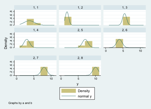
histogram y, by(a b) normal


 
anova y a / b|a /

                     Number of obs =      32     R-squared     =  0.9214
                     Root MSE      = .877971     Adj R-squared =  0.8985

            Source |  Partial SS    df       MS           F     Prob > F
        -----------+----------------------------------------------------
             Model |      217.00     7       31.00      40.22     0.0000
                   |
                 a |      112.50     1      112.50       6.46     0.0440
               b|a |      104.50     6  17.4166667   
        -----------+----------------------------------------------------
               b|a |      104.50     6  17.4166667      22.59     0.0000
                   |
          Residual |       18.50    24  .770833333   
        -----------+----------------------------------------------------
             Total |      235.50    31  7.59677419 
 
regress y x1 x2 x3 x4 x5 x6 x7

  Source |       SS       df       MS               Number of obs =      32
---------+------------------------------            F(  7,    24) =   40.22
   Model |      217.00     7       31.00            Prob > F      =  0.0000
Residual |       18.50    24  .770833333            R-squared     =  0.9214
---------+------------------------------            Adj R-squared =  0.8985
   Total |      235.50    31  7.59677419            Root MSE      =  .87797

------------------------------------------------------------------------------
           y |      Coef.   Std. Err.      t    P>|t|     [95% Conf. Interval]
-------------+----------------------------------------------------------------
          x1 |     -1.875   .1552048   -12.08   0.000    -2.195327   -1.554673
          x2 |          1   .3104097     3.22   0.004     .3593459    1.640654
          x3 |  -.9166667   .1792151    -5.11   0.000    -1.286548   -.5467849
          x4 |   .1666667   .1267242     1.32   0.201    -.0948793    .4282126
          x5 |        1.5   .3104097     4.83   0.000     .8593459    2.140654
          x6 |  -.8333333   .1792151    -4.65   0.000    -1.203215   -.4634515
          x7 |  -.9166667   .1267242    -7.23   0.000    -1.178213   -.6551207
       _cons |      5.375   .1552048    34.63   0.000     5.054673    5.695327
------------------------------------------------------------------------------
 
test2 x1 / x2 x3 x4 x5 x6 x7  /* available from ATS */

Testing: x1 
Error term: x2 x3 x4 x5 x6 x7

     F(  1,   6)  =     6.46
         Prob > F =     0.0440
 
test x2 x3 x4 x5 x6 x7

 ( 1)  x2 = 0.0
 ( 2)  x3 = 0.0
 ( 3)  x4 = 0.0
 ( 4)  x5 = 0.0
 ( 5)  x6 = 0.0
 ( 6)  x7 = 0.0

       F(  6,    24) =   22.59
            Prob > F =    0.0000

Multilevel Model Using xtmixed

It is also possible to analyze these data using a multilevel model approach equivalent to using proc mixed in SAS or using HLM. We will run this as a random intercept restricted maximum likelihood model.

xtmixed y i.a || b: , var /* reml - restricted maximum likelihood model */

Performing EM optimization: 

Performing gradient-based optimization: 

Iteration 0:   log restricted-likelihood =  -50.78963  
Iteration 1:   log restricted-likelihood =  -50.78963  

Computing standard errors:

Mixed-effects REML regression                   Number of obs      =        32
Group variable: b                               Number of groups   =         8

                                                Obs per group: min =         4
                                                               avg =       4.0
                                                               max =         4


                                                Wald chi2(1)       =      6.46
Log restricted-likelihood =  -50.78963          Prob > chi2        =    0.0110

------------------------------------------------------------------------------
           y |      Coef.   Std. Err.      z    P>|z|     [95% Conf. Interval]
-------------+----------------------------------------------------------------
         2.a |       3.75   1.475495     2.54   0.011     .8580829    6.641917
       _cons |        3.5   1.043333     3.35   0.001     1.455106    5.544894
------------------------------------------------------------------------------

------------------------------------------------------------------------------
  Random-effects Parameters  |   Estimate   Std. Err.     [95% Conf. Interval]
-----------------------------+------------------------------------------------
b: Identity                  |
                  var(_cons) |   4.161463   2.514498      1.273271    13.60101
-----------------------------+------------------------------------------------
               var(Residual) |   .7708331   .2225203      .4377636    1.357316
------------------------------------------------------------------------------
LR test vs. linear regression: chibar2(01) =    31.43 Prob >= chibar2 = 0.0000

test 2.a

 ( 1)  [y]2.a = 0

           chi2(  1) =    6.46
         Prob > chi2 =    0.0110

anovalator a, main fratio

anovalator main-effect for a  
chi2(1) = 6.4593237   p-value = .01103716
scaled as F-ratio = 6.4593237

Examples of additional nested models

CRH-pq(A)r(A*B)

Linear Model

Y_ijkl = μ + α_j + β_k(j) + γ_l(jk) + ε_i(jkl)

Schematic

a1 a2
b1 c1 s1
b1 c2 s2
b2 c3 s3
b2 c4 s4
b3 c5 s5
b3 c6 s6
b4 c7 s7
b4 c8 s8

Anova Summary Table for CRH-pq(A)r(A*B) where A is a Fixed Variable
  Source     Errorterm     df
1 A             [2]        p-1
2 B(A)          [3]        p(q_(j)-1)
3 C(A*B)        [4]        pq_(j)(r_(jk)-1)
4 Residual                 pq_(j)r_(jk)(n-1)

CRPH-pq(A)r

Linear Model

Y_ijkl = μ + α_j + β_k(j) + γ_l + αγ_jl + βγ_k(j)l + ε_i(jkl)

Schematic

a1
c1 a1
c2 a2
c1 a2
c2
b1 s1 s3
b2 s2 s4
b3 s5 s7
b4 s6 s8

Anova Summary Table for CRPH-pq(A)r where A & C are Fixed Variables
  Source      Errorterm    df
1 A              [2]       p-1
2 B(A)           [6]       p(q_(j)-1)
3 C              [5]       r-1
4 A*C            [5]       (p-1)(r-1)
5 B(A)*C         [6]       p(q_(j)-1)(r-1)
6 Residual                 pq_(j)r(n-1)

CRPH-pq(A)r(A)

Linear Model

Y_ijkl = μ + α_j + β_k(j) + γ_l(j) + βγ_k(j)l(j) + ε_i(jkl)

Schematic

a1 a2
b1 c1 s1
b1 c2 s2
b2 c1 s3
b2 c2 s4
b3 c3 s5
b3 c4 s6
b4 c3 s7
b4 c4 s8

Anova Summary Table for CRPH-pq(A)r(A) where A & C are Fixed Variables
  Source      Errorterm    df
1 A              [2]       p-1
2 B(A)           [5]       p(q_(j)-1)
3 C(A)           [4]       p(r_(j)-1)
4 B(A)*C(A)      [5]       p(q_(j)-1)(r_(j)-1)
5 Residual                 pq_(j)r_(j)(n-1)

CRPH-pqr(A*B)

Linear Model

Y_ijkl = μ + α_j + β_k + γ_l(jk) + αβ_jk + ε_i(jkl)

Schematic

a1
b1 a1
b2 a2
b1 a2
b2
c1 s1
c2 s2
c3 s3
c4 s4
c5 s5
c6 s6
c7 s7
c8 s8

Anova Summary Table for CRPH-pqr(A*B) where A & B are Fixed Variables
  Source     Errorterm     df
1 A             [3]        p-1
2 B             [3]        q-1
3 C(A*B)        [5]        pq(r_(jk)-1)
4 A*B           [5]        (p-1)(q-1)
5 Residual                 pqr_(jk)(n-1)

Linear Statistical Models Course

Phil Ender, 17sep10, 14may06, 9may00

	a1	a2
b1 c1	s1
b1 c2	s2
b2 c3	s3
b2 c4	s4
b3 c5		s5
b3 c6		s6
b4 c7		s7
b4 c8		s8

	a1	a2
b1 c1	s1
b1 c2	s2
b2 c1	s3
b2 c2	s4
b3 c3		s5
b3 c4		s6
b4 c3		s7
b4 c4		s8