
RBF-pq
Schematic with Example Data
Level s a1 a2 a3
b1 s1
s2
s3
s4
s5
37
42
33
29
24
39
30
34
26
21
31
21
20
18
10
b2 s1
s2
s3
s4
s5
43
44
36
27
25
35
40
31
22
27
41
50
39
36
34
b3 s1
s2
s3
s4
s5
48
47
29
38
28
46
36
45
27
26
64
52
53
42
49
Or in the abbreviated form,
| Level | a1 | a2 | a3 |
| b1 | S1 n = 5 | S1 n = 5 | S1 n = 5 |
| b2 | S1 n = 5 | S1 n = 5 | S1 n = 5 |
| b3 | S1 n = 5 | S1 n = 5 | S1 n = 5 |
Linear Model
Yijk = μ + αj + βk + αβjk + πi + εijk
μ = overall poulation mean
αj = the effect of treatment level j
βk = the effect of treatment level k
αβjk = the joint effects of treatment level j and k
πi = the effect of block i
εijk = experimental error
Hypotheses
Assumptions
| 1. | Independence |
| 2. | Normality |
| 3. | Homogeneity of variance |
| 4. | Non-additivity |
| 5. | Variance-covariance matrix a. compound symmetry b. circularity c. sphericity |
Expected Mean Squares
E(MS a)     = σ2ε + nσ2α
E(MS b)     = σ2ε + nσ2β
E(MS a*b)   = σ2ε + nσs2αβ
E(MS blks)  = σ2ε + pσ2π
E(MS res)   = σ2ε
ANOVA Summary Table
| Source | SS | df | MS | F | p-value | Error | |
| 1 | A | 190.000 | 2 | 95.000 | 4.79 | .0152 | [5] |
| 2 | B | 1543.333 | 2 | 771.666 | 38.99 | .0000 | [5] |
| 3 | A*B | 1236.667 | 4 | 309.167 | 15.58 | .0000 | [5] |
| 4 | Blocks (Subjects) | 1615.111 | 4 | 403.778 | 20.35 | .0000 | [5] |
| 5 | Residual | 634.889 | 32 | 19.840 | |||
| Total | 5220.000 | 44 |
Omega-Squared
ω2A*B = (1236.6667 - 4*19.84)/(634.889 + 19.84) = 0.2209
ω2B = (1543.333 - 2*19.84)/(634.889 + 19.84) = 0.2870
ω2A = (1190.0 - 2*19.84)/(634.889 + 19.84) = 0.0287
Using Stata
input s a b y x1 x2 x3 x4 s1 s2 s3 s4
1 1 1 37 1 1 1 1 1 1 1 1
2 1 1 42 1 1 1 1 -1 1 1 1
3 1 1 33 1 1 1 1 0 -2 1 1
4 1 1 29 1 1 1 1 0 0 -3 1
5 1 1 24 1 1 1 1 0 0 0 -4
1 1 2 43 1 1 -1 1 1 1 1 1
2 1 2 44 1 1 -1 1 -1 1 1 1
3 1 2 36 1 1 -1 1 0 -2 1 1
4 1 2 27 1 1 -1 1 0 0 -3 1
5 1 2 25 1 1 -1 1 0 0 0 -4
1 1 3 48 1 1 0 -2 1 1 1 1
2 1 3 47 1 1 0 -2 -1 1 1 1
3 1 3 29 1 1 0 -2 0 -2 1 1
4 1 3 38 1 1 0 -2 0 0 -3 1
5 1 3 28 1 1 0 -2 0 0 0 -4
1 2 1 39 -1 1 1 1 1 1 1 1
2 2 1 30 -1 1 1 1 -1 1 1 1
3 2 1 34 -1 1 1 1 0 -2 1 1
4 2 1 26 -1 1 1 1 0 0 -3 1
5 2 1 21 -1 1 1 1 0 0 0 -4
1 2 2 35 -1 1 -1 1 1 1 1 1
2 2 2 40 -1 1 -1 1 -1 1 1 1
3 2 2 31 -1 1 -1 1 0 -2 1 1
4 2 2 22 -1 1 -1 1 0 0 -3 1
5 2 2 27 -1 1 -1 1 0 0 0 -4
1 2 3 46 -1 1 0 -2 1 1 1 1
2 2 3 36 -1 1 0 -2 -1 1 1 1
3 2 3 45 -1 1 0 -2 0 -2 1 1
4 2 3 27 -1 1 0 -2 0 0 -3 1
5 2 3 26 -1 1 0 -2 0 0 0 -4
1 3 1 31 0 -2 1 1 1 1 1 1
2 3 1 21 0 -2 1 1 -1 1 1 1
3 3 1 20 0 -2 1 1 0 -2 1 1
4 3 1 18 0 -2 1 1 0 0 -3 1
5 3 1 10 0 -2 1 1 0 0 0 -4
1 3 2 41 0 -2 -1 1 1 1 1 1
2 3 2 50 0 -2 -1 1 -1 1 1 1
3 3 2 39 0 -2 -1 1 0 -2 1 1
4 3 2 36 0 -2 -1 1 0 0 -3 1
5 3 2 34 0 -2 -1 1 0 0 0 -4
1 3 3 64 0 -2 0 -2 1 1 1 1
2 3 3 52 0 -2 0 -2 -1 1 1 1
3 3 3 53 0 -2 0 -2 0 -2 1 1
4 3 3 42 0 -2 0 -2 0 0 -3 1
5 3 3 49 0 -2 0 -2 0 0 0 -4
end
table a, cont(freq mean y sd y) by(b)
----------+-----------------------------------
b and a | Freq. mean(y) sd(y)
----------+-----------------------------------
1 |
1 | 5 33 6.964194
2 | 5 30 6.964194
3 | 5 20 7.516648
----------+-----------------------------------
2 |
1 | 5 35 8.803409
2 | 5 31 6.964194
3 | 5 40 6.204837
----------+-----------------------------------
3 |
1 | 5 38 9.513149
2 | 5 36 9.513149
3 | 5 52 7.968688
----------+-----------------------------------
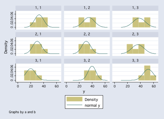
histogram y, by(a b) normal
 anova y a b a#b s, repeated(a b)
Number of obs = 45 R-squared = 0.8784
Root MSE = 4.45424 Adj R-squared = 0.8328
Source | Partial SS df MS F Prob > F
-----------+----------------------------------------------------
Model | 4585.11111 12 382.092593 19.26 0.0000
|
a | 190 2 95 4.79 0.0152
b | 1543.33333 2 771.666667 38.89 0.0000
a#b | 1236.66667 4 309.166667 15.58 0.0000
s | 1615.11111 4 403.777778 20.35 0.0000
|
Residual | 634.888889 32 19.8402778
-----------+----------------------------------------------------
Total | 5220 44 118.636364
Between-subjects error term: s
Levels: 5 (4 df)
Lowest b.s.e. variable: s
Repeated variable: a
Huynh-Feldt epsilon = 0.7892
Greenhouse-Geisser epsilon = 0.6319
Box's conservative epsilon = 0.5000
------------ Prob > F ------------
Source | df F Regular H-F G-G Box
-----------+----------------------------------------------------
a | 2 4.79 0.0152 0.0237 0.0331 0.0438
Residual | 32
----------------------------------------------------------------
Repeated variable: b
Huynh-Feldt epsilon = 0.9493
Greenhouse-Geisser epsilon = 0.6954
Box's conservative epsilon = 0.5000
------------ Prob > F ------------
Source | df F Regular H-F G-G Box
-----------+----------------------------------------------------
b | 2 38.89 0.0000 0.0000 0.0000 0.0000
Residual | 32
----------------------------------------------------------------
Repeated variables: a#b
Huynh-Feldt epsilon = 1.4947
*Huynh-Feldt epsilon reset to 1.0000
Greenhouse-Geisser epsilon = 0.5901
Box's conservative epsilon = 0.2500
------------ Prob > F ------------
Source | df F Regular H-F G-G Box
-----------+----------------------------------------------------
a#b | 4 15.58 0.0000 0.0000 0.0001 0.0043
Residual | 32
----------------------------------------------------------------
effectsize a#b
anova effect size for a#b with dep var = y
total variance accounted for
omega2 = .22086657
eta2 = .23690932
Cohen's f = .53242578
partial variance accounted for
partial omega2 = .56450679
partial eta2 = .66076941
effectsize b
anova effect size for b with dep var = y
total variance accounted for
omega2 = .28696538
eta2 = .29565773
Cohen's f = .63439456
partial variance accounted for
partial omega2 = .62744609
partial eta2 = .70852887
effectsize a
anova effect size for a with dep var = y
total variance accounted for
omega2 = .02868779
eta2 = .03639847
Cohen's f = .17185775
partial variance accounted for
partial omega2 = .14410396
partial eta2 = .23033405
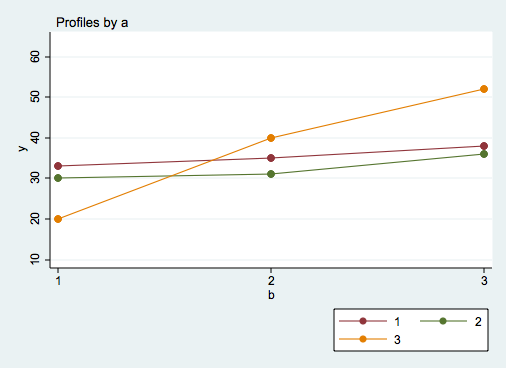
quietly anova y a b a#b /* run without s to get a plot of cell means */
anovaplot b a, scatter(msym(none))
anova y a b a#b s, repeated(a b)
Number of obs = 45 R-squared = 0.8784
Root MSE = 4.45424 Adj R-squared = 0.8328
Source | Partial SS df MS F Prob > F
-----------+----------------------------------------------------
Model | 4585.11111 12 382.092593 19.26 0.0000
|
a | 190 2 95 4.79 0.0152
b | 1543.33333 2 771.666667 38.89 0.0000
a#b | 1236.66667 4 309.166667 15.58 0.0000
s | 1615.11111 4 403.777778 20.35 0.0000
|
Residual | 634.888889 32 19.8402778
-----------+----------------------------------------------------
Total | 5220 44 118.636364
Between-subjects error term: s
Levels: 5 (4 df)
Lowest b.s.e. variable: s
Repeated variable: a
Huynh-Feldt epsilon = 0.7892
Greenhouse-Geisser epsilon = 0.6319
Box's conservative epsilon = 0.5000
------------ Prob > F ------------
Source | df F Regular H-F G-G Box
-----------+----------------------------------------------------
a | 2 4.79 0.0152 0.0237 0.0331 0.0438
Residual | 32
----------------------------------------------------------------
Repeated variable: b
Huynh-Feldt epsilon = 0.9493
Greenhouse-Geisser epsilon = 0.6954
Box's conservative epsilon = 0.5000
------------ Prob > F ------------
Source | df F Regular H-F G-G Box
-----------+----------------------------------------------------
b | 2 38.89 0.0000 0.0000 0.0000 0.0000
Residual | 32
----------------------------------------------------------------
Repeated variables: a#b
Huynh-Feldt epsilon = 1.4947
*Huynh-Feldt epsilon reset to 1.0000
Greenhouse-Geisser epsilon = 0.5901
Box's conservative epsilon = 0.2500
------------ Prob > F ------------
Source | df F Regular H-F G-G Box
-----------+----------------------------------------------------
a#b | 4 15.58 0.0000 0.0000 0.0001 0.0043
Residual | 32
----------------------------------------------------------------
effectsize a#b
anova effect size for a#b with dep var = y
total variance accounted for
omega2 = .22086657
eta2 = .23690932
Cohen's f = .53242578
partial variance accounted for
partial omega2 = .56450679
partial eta2 = .66076941
effectsize b
anova effect size for b with dep var = y
total variance accounted for
omega2 = .28696538
eta2 = .29565773
Cohen's f = .63439456
partial variance accounted for
partial omega2 = .62744609
partial eta2 = .70852887
effectsize a
anova effect size for a with dep var = y
total variance accounted for
omega2 = .02868779
eta2 = .03639847
Cohen's f = .17185775
partial variance accounted for
partial omega2 = .14410396
partial eta2 = .23033405
quietly anova y a b a#b /* run without s to get a plot of cell means */
anovaplot b a, scatter(msym(none))
 quietly anova y a b a#b s /* rerun the original anova to get correct mse */
sme a b
Test of a at b(1): F(2/32) = 11.676584
Test of a at b(2): F(2/32) = 5.1242562
Test of a at b(3): F(2/32) = 19.152958
Critical value of F for alpha = .05 using ...
--------------------------------------------------
Dunn's procedure = 4.1487813
Marascuilo & Levin = 4.6658516
per family error rate = 4.6658516
simultaneous test procedure = 9.4358325
anovalator a b, simple fratio
anovalator test of simple main effects for a at(b=1)
chi2(2) = 23.353168 p-value = 8.490e-06
scaled as F-ratio = 11.676584
anovalator test of simple main effects for a at(b=2)
chi2(2) = 10.248512 p-value = .00595064
scaled as F-ratio = 5.1242562
anovalator test of simple main effects for a at(b=3)
chi2(2) = 38.305915 p-value = 4.808e-09
scaled as F-ratio = 19.152958
smecriticalvalue, num(3) df1(2) df2(32) dfm(12)
number of tests: 3
numerator df: 2
denominator df: 32
original model df: 12
Critical value of F for alpha = .05 using ...
------------------------------------------------
Dunn's procedure = 5.0408416
Marascuilo & Levin = 5.5808631
per family error rate = 4.6659053
simultaneous test procedure = 9.435821
tkcomp a if b==1
Tukey-Kramer pairwise comparisons for variable a
studentized range critical value(.05, 3, 32) = 3.4754008
mean
grp vs grp group means dif TK-test
-------------------------------------------------------
1 vs 2 33.0000 30.0000 3.0000 1.5060
1 vs 3 33.0000 20.0000 13.0000 6.5261*
2 vs 3 30.0000 20.0000 10.0000 5.0201*
tkcomp a if b==3
Tukey-Kramer pairwise comparisons for variable a
studentized range critical value(.05, 3, 32) = 3.4754008
mean
grp vs grp group means dif TK-test
-------------------------------------------------------
1 vs 2 38.0000 36.0000 2.0000 1.0040
1 vs 3 38.0000 52.0000 14.0000 7.0281*
2 vs 3 36.0000 52.0000 16.0000 8.0321*
anovalator a, pair at(b=1) quietly
anovalator pairwise comparisons for a at(b=1)
Comparison Coef. Std. Err. z P>|z| [95% Conf. Interval]
1 vs 2 3 2.81711 1.06 0.287 -2.521536 8.521536
1 vs 3 13 2.81711 4.61 0.000 7.478464 18.52154
2 vs 3 10 2.81711 3.55 0.000 4.478464 15.52154
anovalator a, pair at(b=3) quietly
anovalator pairwise comparisons for a at(b=3)
Comparison Coef. Std. Err. z P>|z| [95% Conf. Interval]
1 vs 2 2 2.81711 .71 0.478 -3.521536 7.521536
1 vs 3 -14 2.81711 -4.97 0.000 -19.52154 -8.478464
2 vs 3 -16 2.81711 -5.68 0.000 -21.52154 -10.47846
generate x5 = x1*x3
generate x6 = x1*x4
generate x7 = x2*x3
generate x8 = x2*x4
regress y x1 x2 x3 x4 x5 x6 x7 x8 s1 s2 s3 s4
Source | SS df MS Number of obs = 45
-------------+------------------------------ F( 12, 32) = 19.26
Model | 4585.11111 12 382.092593 Prob > F = 0.0000
Residual | 634.888889 32 19.8402778 R-squared = 0.8784
-------------+------------------------------ Adj R-squared = 0.8328
Total | 5220 44 118.636364 Root MSE = 4.4542
------------------------------------------------------------------------------
y | Coef. Std. Err. t P>|t| [95% Conf. Interval]
-------------+----------------------------------------------------------------
x1 | 1.5 .8132297 1.84 0.074 -.1564948 3.156495
x2 | -1.166667 .4695184 -2.48 0.018 -2.123044 -.210289
x3 | -3.833333 .8132297 -4.71 0.000 -5.489828 -2.176839
x4 | -3.5 .4695184 -7.45 0.000 -4.456378 -2.543622
x5 | -.25 .9959989 -0.25 0.803 -2.278783 1.778783
x6 | .25 .5750403 0.43 0.667 -.9213187 1.421319
x7 | 3.083333 .5750403 5.36 0.000 1.912015 4.254652
x8 | 1.916667 .3319996 5.77 0.000 1.240406 2.592928
s1 | 1.222222 1.049875 1.16 0.253 -.9163033 3.360748
s2 | 1.962963 .6061457 3.24 0.003 .7282847 3.197641
s3 | 2.509259 .4286097 5.85 0.000 1.63621 3.382309
s4 | 1.972222 .3319996 5.94 0.000 1.295961 2.648483
_cons | 35 .6639993 52.71 0.000 33.64748 36.35252
------------------------------------------------------------------------------
test x1 x2
( 1) x1 = 0
( 2) x2 = 0
F( 2, 32) = 4.79
Prob > F = 0.0152
test x3 x4
( 1) x3 = 0
( 2) x4 = 0
F( 2, 32) = 38.89
Prob > F = 0.0000
test x5 x6 x7 x8
( 1) x5 = 0
( 2) x6 = 0
( 3) x7 = 0
( 4) x8 = 0
F( 4, 32) = 15.58
Prob > F = 0.0000
test s1 s2 s3 s4
( 1) s1 = 0
( 2) s2 = 0
( 3) s3 = 0
( 4) s4 = 0
F( 4, 32) = 20.35
Prob > F = 0.0000
regress y i.a##i.b i.s
Source | SS df MS Number of obs = 45
-------------+------------------------------ F( 12, 32) = 19.26
Model | 4585.11111 12 382.092593 Prob > F = 0.0000
Residual | 634.888889 32 19.8402778 R-squared = 0.8784
-------------+------------------------------ Adj R-squared = 0.8328
Total | 5220 44 118.636364 Root MSE = 4.4542
------------------------------------------------------------------------------
y | Coef. Std. Err. t P>|t| [95% Conf. Interval]
-------------+----------------------------------------------------------------
a |
2 | -3 2.81711 -1.06 0.295 -8.738266 2.738266
3 | -13 2.81711 -4.61 0.000 -18.73827 -7.261734
|
b |
2 | 2 2.81711 0.71 0.483 -3.738266 7.738266
3 | 5 2.81711 1.77 0.085 -.7382661 10.73827
|
a#b |
2 2 | -1 3.983996 -0.25 0.803 -9.115134 7.115134
2 3 | 1 3.983996 0.25 0.803 -7.115134 9.115134
3 2 | 18 3.983996 4.52 0.000 9.884866 26.11513
3 3 | 27 3.983996 6.78 0.000 18.88487 35.11513
|
s |
2 | -2.444444 2.09975 -1.16 0.253 -6.721496 1.832607
3 | -7.111111 2.09975 -3.39 0.002 -11.38816 -2.83406
4 | -13.22222 2.09975 -6.30 0.000 -17.49927 -8.945171
5 | -15.55556 2.09975 -7.41 0.000 -19.83261 -11.2785
|
_cons | 40.66667 2.394083 16.99 0.000 35.79008 45.54326
------------------------------------------------------------------------------
anovalator a b, main 2way fratio
anovalator main-effect for a
chi2(2) = 9.5764788 p-value = .00832711
scaled as F-ratio = 4.7882394
anovalator main-effect for b
chi2(2) = 77.787889 p-value = 1.284e-17
scaled as F-ratio = 38.893945
anovalator two-way interaction for a#b
chi2(4) = 62.331117 p-value = 9.383e-13
scaled as F-ratio = 15.582779
anovalator s, main fratio
anovalator main-effect for s
chi2(4) = 81.40567 p-value = 8.773e-17
scaled as F-ratio = 20.351418
quietly anova y a b a#b s /* rerun the original anova to get correct mse */
sme a b
Test of a at b(1): F(2/32) = 11.676584
Test of a at b(2): F(2/32) = 5.1242562
Test of a at b(3): F(2/32) = 19.152958
Critical value of F for alpha = .05 using ...
--------------------------------------------------
Dunn's procedure = 4.1487813
Marascuilo & Levin = 4.6658516
per family error rate = 4.6658516
simultaneous test procedure = 9.4358325
anovalator a b, simple fratio
anovalator test of simple main effects for a at(b=1)
chi2(2) = 23.353168 p-value = 8.490e-06
scaled as F-ratio = 11.676584
anovalator test of simple main effects for a at(b=2)
chi2(2) = 10.248512 p-value = .00595064
scaled as F-ratio = 5.1242562
anovalator test of simple main effects for a at(b=3)
chi2(2) = 38.305915 p-value = 4.808e-09
scaled as F-ratio = 19.152958
smecriticalvalue, num(3) df1(2) df2(32) dfm(12)
number of tests: 3
numerator df: 2
denominator df: 32
original model df: 12
Critical value of F for alpha = .05 using ...
------------------------------------------------
Dunn's procedure = 5.0408416
Marascuilo & Levin = 5.5808631
per family error rate = 4.6659053
simultaneous test procedure = 9.435821
tkcomp a if b==1
Tukey-Kramer pairwise comparisons for variable a
studentized range critical value(.05, 3, 32) = 3.4754008
mean
grp vs grp group means dif TK-test
-------------------------------------------------------
1 vs 2 33.0000 30.0000 3.0000 1.5060
1 vs 3 33.0000 20.0000 13.0000 6.5261*
2 vs 3 30.0000 20.0000 10.0000 5.0201*
tkcomp a if b==3
Tukey-Kramer pairwise comparisons for variable a
studentized range critical value(.05, 3, 32) = 3.4754008
mean
grp vs grp group means dif TK-test
-------------------------------------------------------
1 vs 2 38.0000 36.0000 2.0000 1.0040
1 vs 3 38.0000 52.0000 14.0000 7.0281*
2 vs 3 36.0000 52.0000 16.0000 8.0321*
anovalator a, pair at(b=1) quietly
anovalator pairwise comparisons for a at(b=1)
Comparison Coef. Std. Err. z P>|z| [95% Conf. Interval]
1 vs 2 3 2.81711 1.06 0.287 -2.521536 8.521536
1 vs 3 13 2.81711 4.61 0.000 7.478464 18.52154
2 vs 3 10 2.81711 3.55 0.000 4.478464 15.52154
anovalator a, pair at(b=3) quietly
anovalator pairwise comparisons for a at(b=3)
Comparison Coef. Std. Err. z P>|z| [95% Conf. Interval]
1 vs 2 2 2.81711 .71 0.478 -3.521536 7.521536
1 vs 3 -14 2.81711 -4.97 0.000 -19.52154 -8.478464
2 vs 3 -16 2.81711 -5.68 0.000 -21.52154 -10.47846
generate x5 = x1*x3
generate x6 = x1*x4
generate x7 = x2*x3
generate x8 = x2*x4
regress y x1 x2 x3 x4 x5 x6 x7 x8 s1 s2 s3 s4
Source | SS df MS Number of obs = 45
-------------+------------------------------ F( 12, 32) = 19.26
Model | 4585.11111 12 382.092593 Prob > F = 0.0000
Residual | 634.888889 32 19.8402778 R-squared = 0.8784
-------------+------------------------------ Adj R-squared = 0.8328
Total | 5220 44 118.636364 Root MSE = 4.4542
------------------------------------------------------------------------------
y | Coef. Std. Err. t P>|t| [95% Conf. Interval]
-------------+----------------------------------------------------------------
x1 | 1.5 .8132297 1.84 0.074 -.1564948 3.156495
x2 | -1.166667 .4695184 -2.48 0.018 -2.123044 -.210289
x3 | -3.833333 .8132297 -4.71 0.000 -5.489828 -2.176839
x4 | -3.5 .4695184 -7.45 0.000 -4.456378 -2.543622
x5 | -.25 .9959989 -0.25 0.803 -2.278783 1.778783
x6 | .25 .5750403 0.43 0.667 -.9213187 1.421319
x7 | 3.083333 .5750403 5.36 0.000 1.912015 4.254652
x8 | 1.916667 .3319996 5.77 0.000 1.240406 2.592928
s1 | 1.222222 1.049875 1.16 0.253 -.9163033 3.360748
s2 | 1.962963 .6061457 3.24 0.003 .7282847 3.197641
s3 | 2.509259 .4286097 5.85 0.000 1.63621 3.382309
s4 | 1.972222 .3319996 5.94 0.000 1.295961 2.648483
_cons | 35 .6639993 52.71 0.000 33.64748 36.35252
------------------------------------------------------------------------------
test x1 x2
( 1) x1 = 0
( 2) x2 = 0
F( 2, 32) = 4.79
Prob > F = 0.0152
test x3 x4
( 1) x3 = 0
( 2) x4 = 0
F( 2, 32) = 38.89
Prob > F = 0.0000
test x5 x6 x7 x8
( 1) x5 = 0
( 2) x6 = 0
( 3) x7 = 0
( 4) x8 = 0
F( 4, 32) = 15.58
Prob > F = 0.0000
test s1 s2 s3 s4
( 1) s1 = 0
( 2) s2 = 0
( 3) s3 = 0
( 4) s4 = 0
F( 4, 32) = 20.35
Prob > F = 0.0000
regress y i.a##i.b i.s
Source | SS df MS Number of obs = 45
-------------+------------------------------ F( 12, 32) = 19.26
Model | 4585.11111 12 382.092593 Prob > F = 0.0000
Residual | 634.888889 32 19.8402778 R-squared = 0.8784
-------------+------------------------------ Adj R-squared = 0.8328
Total | 5220 44 118.636364 Root MSE = 4.4542
------------------------------------------------------------------------------
y | Coef. Std. Err. t P>|t| [95% Conf. Interval]
-------------+----------------------------------------------------------------
a |
2 | -3 2.81711 -1.06 0.295 -8.738266 2.738266
3 | -13 2.81711 -4.61 0.000 -18.73827 -7.261734
|
b |
2 | 2 2.81711 0.71 0.483 -3.738266 7.738266
3 | 5 2.81711 1.77 0.085 -.7382661 10.73827
|
a#b |
2 2 | -1 3.983996 -0.25 0.803 -9.115134 7.115134
2 3 | 1 3.983996 0.25 0.803 -7.115134 9.115134
3 2 | 18 3.983996 4.52 0.000 9.884866 26.11513
3 3 | 27 3.983996 6.78 0.000 18.88487 35.11513
|
s |
2 | -2.444444 2.09975 -1.16 0.253 -6.721496 1.832607
3 | -7.111111 2.09975 -3.39 0.002 -11.38816 -2.83406
4 | -13.22222 2.09975 -6.30 0.000 -17.49927 -8.945171
5 | -15.55556 2.09975 -7.41 0.000 -19.83261 -11.2785
|
_cons | 40.66667 2.394083 16.99 0.000 35.79008 45.54326
------------------------------------------------------------------------------
anovalator a b, main 2way fratio
anovalator main-effect for a
chi2(2) = 9.5764788 p-value = .00832711
scaled as F-ratio = 4.7882394
anovalator main-effect for b
chi2(2) = 77.787889 p-value = 1.284e-17
scaled as F-ratio = 38.893945
anovalator two-way interaction for a#b
chi2(4) = 62.331117 p-value = 9.383e-13
scaled as F-ratio = 15.582779
anovalator s, main fratio
anovalator main-effect for s
chi2(4) = 81.40567 p-value = 8.773e-17
scaled as F-ratio = 20.351418
Linear Statistical Models Course
Phil Ender, 17sep10, 25apr06, 12Feb98