Assumptions

1.	Independence
2.	Normality
3.	Homogeneity of variance
4.	No Non-additivity (no block*treatment interaction)
5.	Compound symmetry in the variance-covariance matrix

ANOVA Summary Table

	Source	SS	df	MS	F	p-value	Error
1	Treatment	49.00	3	16.33	11.63	0.0001	[3]
2	Blocks (Subjects)	31.50	7	4.50	3.20	0.0180	[3]
3	Residual	29.50	21	1.40
	Total	110.00	31

Table of the F-distribution

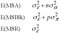
Expected Mean Squares

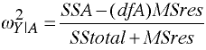
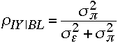
Strength of Association

Using Stata: Method 1

input y a s x1 x2 x3 s1 s2 s3 s4 s5 s6 s7
 3 1 1  1  1  1  1  1  1  1  1  1  1
 2 1 2  1  1  1 -1  1  1  1  1  1  1
 2 1 3  1  1  1  0 -2  1  1  1  1  1
 3 1 4  1  1  1  0  0 -3  1  1  1  1
 1 1 5  1  1  1  0  0  0 -4  1  1  1
 3 1 6  1  1  1  0  0  0  0 -5  1  1
 4 1 7  1  1  1  0  0  0  0  0 -6  1
 6 1 8  1  1  1  0  0  0  0  0  0 -7
 4 2 1 -1  1  1  1  1  1  1  1  1  1
 4 2 2 -1  1  1 -1  1  1  1  1  1  1 
 3 2 3 -1  1  1  0 -2  1  1  1  1  1
 3 2 4 -1  1  1  0  0 -3  1  1  1  1
 2 2 5 -1  1  1  0  0  0 -4  1  1  1
 3 2 6 -1  1  1  0  0  0  0 -5  1  1
 4 2 7 -1  1  1  0  0  0  0  0 -6  1
 5 2 8 -1  1  1  0  0  0  0  0  0 -7
 4 3 1  0 -2  1  1  1  1  1  1  1  1
 4 3 2  0 -2  1 -1  1  1  1  1  1  1
 3 3 3  0 -2  1  0 -2  1  1  1  1  1
 3 3 4  0 -2  1  0  0 -3  1  1  1  1
 4 3 5  0 -2  1  0  0  0 -4  1  1  1
 6 3 6  0 -2  1  0  0  0  0 -5  1  1
 5 3 7  0 -2  1  0  0  0  0  0 -6  1
 5 3 8  0 -2  1  0  0  0  0  0  0 -7
 3 4 1  0  0 -3  1  1  1  1  1  1  1
 5 4 2  0  0 -3 -1  1  1  1  1  1  1
 6 4 3  0  0 -3  0 -2  1  1  1  1  1
 5 4 4  0  0 -3  0  0 -3  1  1  1  1
 7 4 5  0  0 -3  0  0  0 -4  1  1  1
 6 4 6  0  0 -3  0  0  0  0 -5  1  1
10 4 7  0  0 -3  0  0  0  0  0 -6  1
 8 4 8  0  0 -3  0  0  0  0  0  0 -7
end
  
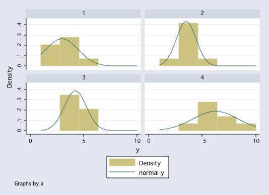
tabstat y, by(a) stat(n mean sd var)

Summary for variables: y
     by categories of: a 

       a |         N      mean        sd  variance
---------+----------------------------------------
       1 |         8         3  1.511858  2.285714
       2 |         8       3.5  .9258201  .8571429
       3 |         8      4.25  1.035098  1.071429
       4 |         8      6.25   2.12132       4.5
---------+----------------------------------------
   Total |        32      4.25  1.883716  3.548387
--------------------------------------------------
  
histogram y, by(a) normal
  

  
anova y a s, repeated(a)

                           Number of obs =      32     R-squared     =  0.7318
                           Root MSE      = 1.18523     Adj R-squared =  0.6041

                  Source |  Partial SS    df       MS           F     Prob > F
              -----------+----------------------------------------------------
                   Model |       80.50    10        8.05       5.73     0.0004
                         |
                       a |       49.00     3  16.3333333      11.63     0.0001
                       s |       31.50     7        4.50       3.20     0.0180
                         |
                Residual |       29.50    21   1.4047619   
              -----------+----------------------------------------------------
                   Total |      110.00    31   3.5483871   


Between-subjects error term:  s
                     Levels:  8         (7 df)
     Lowest b.s.e. variable:  s

Repeated variable: a
                                          Huynh-Feldt epsilon        =  0.8343
                                          Greenhouse-Geisser epsilon =  0.6195
                                          Box's conservative epsilon =  0.3333

                                            ------------ Prob > F ------------
                  Source |     df      F    Regular    H-F      G-G      Box
              -----------+----------------------------------------------------
                       a |      3    11.63   0.0001   0.0003   0.0015   0.0113
                Residual |     21
              -----------+----------------------------------------------------
  
mat list e(Srep)
  
symmetric e(Srep)[4,4]
           c1         c2         c3         c4
r1  2.2857143
r2  1.1428571  .85714286
r3  .71428571  .28571429  1.0714286
r4  1.2857143  .28571429  .92857143        4.5
  
effectsize a

anova effect size for a with dep var = y

total variance accounted for
omega2         = .40200898
eta2           = .44545455
Cohen's f      = .81991823

partial variance accounted for
partial omega2 = .49907137
partial eta2   = .62420382
  
nonadd y a s
  
Tukey's test of nonadditivity for randomized block designs
Ho: model is additive (no block*treatment interaction)
F (1,20) = 1.2795813   Pr > F: .27135918
  
 
quietly anova y a s /* quietly rerun anova to get correct mse */
 
tkcomp a
  
Tukey-Kramer pairwise comparisons for variable a
studentized range critical value(.05, 4, 21) = 3.9419483

                                      mean 
grp vs grp       group means          dif     TK-test
-------------------------------------------------------
  1 vs   2     3.0000     3.5000      0.5000   1.1932 
  1 vs   3     3.0000     4.2500      1.2500   2.9830 
  1 vs   4     3.0000     6.2500      3.2500   7.7558*
  2 vs   3     3.5000     4.2500      0.7500   1.7898 
  2 vs   4     3.5000     6.2500      2.7500   6.5626*
  3 vs   4     4.2500     6.2500      2.0000   4.7728*

tukeyhsd a

Tukey HSD pairwise comparisons for variable a
studentized range critical value(.05, 4, 21) = 3.9419483
uses harmonica mean sample size =    8.000

                                      mean     critical
grp vs grp       group means          dif        dif
-------------------------------------------------------
  1 vs   2     3.0000     3.5000     0.5000    1.6518
  1 vs   3     3.0000     4.2500     1.2500    1.6518
  1 vs   4     3.0000     6.2500     3.2500*   1.6518
  2 vs   3     3.5000     4.2500     0.7500    1.6518
  2 vs   4     3.5000     6.2500     2.7500*   1.6518
  3 vs   4     4.2500     6.2500     2.0000*   1.6518
  
regress y x1 x2 x3 s1 s2 s3 s4 s5 s6 s7
  
      Source |       SS       df       MS              Number of obs =      32
-------------+------------------------------           F( 10,    21) =    5.73
       Model |       80.50    10        8.05           Prob > F      =  0.0004
    Residual |       29.50    21   1.4047619           R-squared     =  0.7318
-------------+------------------------------           Adj R-squared =  0.6041
       Total |      110.00    31   3.5483871           Root MSE      =  1.1852

------------------------------------------------------------------------------
           y |      Coef.   Std. Err.      t    P>|t|     [95% Conf. Interval]
-------------+----------------------------------------------------------------
          x1 |       -.25   .2963066    -0.84   0.408    -.8662034    .3662034
          x2 |  -.3333333   .1710727    -1.95   0.065    -.6890985    .0224318
          x3 |  -.6666667   .1209667    -5.51   0.000    -.9182306   -.4151027
          s1 |      -.125   .4190409    -0.30   0.768    -.9964432    .7464432
          s2 |   .0416667   .2419334     0.17   0.865    -.4614613    .5447946
          s3 |   .0208333   .1710727     0.12   0.904    -.3349318    .3765985
          s4 |      .0125   .1325124     0.09   0.926    -.2630745    .2880745
          s5 |  -.1583333   .1081959    -1.46   0.158     -.383339    .0666723
          s6 |  -.2916667   .0914422    -3.19   0.004    -.4818312   -.1015022
          s7 |       -.25   .0791913    -3.16   0.005    -.4146873   -.0853127
       _cons |       4.25   .2095204    20.28   0.000     3.814278    4.685722
------------------------------------------------------------------------------
  
test x1 x2 x3

 ( 1)  x1 = 0.0
 ( 2)  x2 = 0.0
 ( 3)  x3 = 0.0

       F(  3,    21) =   11.63
            Prob > F =    0.0001
       
test s1 s2 s3 s4 s5 s6 s7

 ( 1)  s1 = 0.0
 ( 2)  s2 = 0.0
 ( 3)  s3 = 0.0
 ( 4)  s4 = 0.0
 ( 5)  s5 = 0.0
 ( 6)  s6 = 0.0
 ( 7)  s7 = 0.0

       F(  7,    21) =    3.20
            Prob > F =    0.0180
  
regress y i.a i.s

      Source |       SS       df       MS              Number of obs =      32
-------------+------------------------------           F( 10,    21) =    5.73
       Model |        80.5    10        8.05           Prob > F      =  0.0004
    Residual |        29.5    21   1.4047619           R-squared     =  0.7318
-------------+------------------------------           Adj R-squared =  0.6041
       Total |         110    31   3.5483871           Root MSE      =  1.1852

------------------------------------------------------------------------------
           y |      Coef.   Std. Err.      t    P>|t|     [95% Conf. Interval]
-------------+----------------------------------------------------------------
           a |
          2  |         .5   .5926133     0.84   0.408    -.7324067    1.732407
          3  |       1.25   .5926133     2.11   0.047     .0175933    2.482407
          4  |       3.25   .5926133     5.48   0.000     2.017593    4.482407
             |
           s |
          2  |        .25   .8380817     0.30   0.768    -1.492886    1.992886
          3  |  -1.78e-16   .8380817    -0.00   1.000    -1.742886    1.742886
          4  |  -3.41e-16   .8380817    -0.00   1.000    -1.742886    1.742886
          5  |  -1.86e-16   .8380817    -0.00   1.000    -1.742886    1.742886
          6  |          1   .8380817     1.19   0.246    -.7428863    2.742886
          7  |       2.25   .8380817     2.68   0.014     .5071137    3.992886
          8  |        2.5   .8380817     2.98   0.007     .7571137    4.242886
             |
       _cons |       2.25   .6949006     3.24   0.004      .804875    3.695125
------------------------------------------------------------------------------
  
/* user written program -- findit anovalator */

anovalator a s, main fratio

anovalator main-effect for a  
chi2(3) = 34.881356   p-value = 1.291e-07
scaled as F-ratio = 11.627119

anovalator main-effect for s  
chi2(7) = 22.423729   p-value = .00214632
scaled as F-ratio = 3.2033898

Using Stata: Method 2

Randomized block data often come in a wide form, in which, each of the repeated measures is a separate variable. Before you can alanlyze these data using the Stata anova command you need to reshape the data into a long form. While the data are still wide you can compute the correlation and covariance matrices using the corr command.

input s y1 y2 y3 y4
1  3  4  4  3
2  2  4  4  5
3  2  3  3  6
4  3  3  3  5
5  1  2  4  7
6  3  3  6  6
7  4  4  5 10
8  6  5  5  8
end

corr y1 y2 y3 y4, cov  /* note: covariance matrix same as e(Srep) */

(obs=8)

         |       y1       y2       y3       y4
---------+------------------------------------
          y1 |  2.28571
          y2 |  1.14286  .857143
          y3 |  .714286  .285714  1.07143
          y4 |  1.28571  .285714  .928571      4.5
  
corr y1 y2 y3 y4
(obs=8)

             |       y1       y2       y3       y4
-------------+------------------------------------
          y1 |   1.0000
          y2 |   0.8165   1.0000
          y3 |   0.4564   0.2981   1.0000
          y4 |   0.4009   0.1455   0.4229   1.0000
  
reshape long y, i(s) j(a)

(note:  j = 1 2 3 4)

Data                               wide   ->   long
-----------------------------------------------------------------------------
Number of obs.                        8   ->      32
Number of variables                   5   ->       3
j variable (4 values)                     ->   a
xij variables:
                           y1 y2 ... y4   ->   y
-----------------------------------------------------------------------------
  
list

[output omitted]
  
anova y a s, repeated(a)

                           Number of obs =      32     R-squared     =  0.7318
                           Root MSE      = 1.18523     Adj R-squared =  0.6041

                  Source |  Partial SS    df       MS           F     Prob > F
              -----------+----------------------------------------------------
                   Model |       80.50    10        8.05       5.73     0.0004
                         |
                       a |       49.00     3  16.3333333      11.63     0.0001
                       s |       31.50     7        4.50       3.20     0.0180
                         |
                Residual |       29.50    21   1.4047619   
              -----------+----------------------------------------------------
                   Total |      110.00    31   3.5483871   


Between-subjects error term:  s
                     Levels:  8         (7 df)
     Lowest b.s.e. variable:  s

Repeated variable: a
                                          Huynh-Feldt epsilon        =  0.8343
                                          Greenhouse-Geisser epsilon =  0.6195
                                          Box's conservative epsilon =  0.3333

                                            ------------ Prob > F ------------
                  Source |     df      F    Regular    H-F      G-G      Box
              -----------+----------------------------------------------------
                       a |      3    11.63   0.0001   0.0003   0.0015   0.0113
                Residual |     21
              -----------+----------------------------------------------------

The linear model that is nonadditive would look as follows;

Y_ij = μ + α_j + π_i + απ_ij + ε_ij

One obvious problem is that απ_ij & ε_ij cannot exist as separate entities. The expected mean squares in the nonadditive model are as follows:

E(MSA)   σ²_ε + nσ²_α
E(MSBlk) σ²_ε + pσ²_π
E(MSRes) σ²_ε + σ²_απ

Using the MSRes as the error term, in a nonadditive model, in the F-ratios for treatment and blocks tends to negatively bias the F-ratio. Tukey (1949) came up with a relatively simple test of additivity. This test examines a one degree of freedom linear*linear interaction to test for the presence of nonadditivity. The Tukey test can be run using the Stata nonadd command from ATS.

Using Stata to Obtain Tukey's Test of Additivity

use http://www.philender.com/courses/data/rb4new, clear
  
anova y a s, repeated(a)

                           Number of obs =      32     R-squared     =  0.7318
                           Root MSE      = 1.18523     Adj R-squared =  0.6041

                  Source |  Partial SS    df       MS           F     Prob > F
              -----------+----------------------------------------------------
                   Model |       80.50    10        8.05       5.73     0.0004
                         |
                       a |       49.00     3  16.3333333      11.63     0.0001
                       s |       31.50     7        4.50       3.20     0.0180
                         |
                Residual |       29.50    21   1.4047619   
              -----------+----------------------------------------------------
                   Total |      110.00    31   3.5483871   


Between-subjects error term:  s
                     Levels:  8         (7 df)
     Lowest b.s.e. variable:  s

Repeated variable: a
                                          Huynh-Feldt epsilon        =  0.8343
                                          Greenhouse-Geisser epsilon =  0.6195
                                          Box's conservative epsilon =  0.3333

                                            ------------ Prob > F ------------
                  Source |     df      F    Regular    H-F      G-G      Box
              -----------+----------------------------------------------------
                       a |      3    11.63   0.0001   0.0003   0.0015   0.0113
                Residual |     21
              -----------+----------------------------------------------------

  
nonadd y a s

Tukey's test of nonadditivity for randomized block designs
Ho: model is additive (no block*treatment interaction)
F (1,20) = 1.2795813   Pr > F: .27135918

Blocking

Blocking can be used to hold a nuisance variable constant. In testing math performance, one could block on reading ability by matching subjects on reading test scores. Then each subject within a block is randomly assigned to one of several treatment groups.

Carrying matching to an extreme occurs when the subjects themselves become the block. This is a repeated measures type design.

Counter Balancing

When a randomized block design is used to analyze repeated measures type data, care should be taken to counter balance the order of the treatment so as to eliminate the possibility of order effects in final results. Counter balancing cannot, of course, be done when time is the repeated factor.

Variance-Covariance Matrices

The variance-covariance matrix for the repeated effect can take on any several different forms. Here are some examples:

Independence - 1 parameter

σ2
0  σ2
0  0  σ2

Compound Symmetry - 2 parameters

σ2
σ1  σ2
σ1  σ1  σ2

Autoregressive - 3 parameters

σ2 
σρ   σ2 
σρ2  σρ   σ2 

Unstructured - 6 parameters

σ12
σ12  σ22
σ13  σ23  σ32

The independence covariance structure is typically found in between subject designs with random sampling and random assignment. When the assumption of independence is met the covariance matrix will have zeros or near zeros in the off diagonals. When the assumption of homogeneity of variance is met the diagonal values will all be equal or nearly equal.

Compound symmetry is often found in repeated measures designs which are not time dependent. If the order of the responses does not matter than the covariances are exchangable. The term exchangable is synonymous with compound symmetry. You may also hear the terms spherical or circular which are mathematical measures equating to compound symmetry.

If the response variable is measured at different time points an autoregressive covariance structure often results, in which, observations more closely associated in time are more strongly correlated than observations farther apart in time.

Finally, when there does not seem to be any discernable pattern in the covariance matrix the matrix is said to be unstructured. The multivariate option below makes use of an unstructured covariance matrix.

The Compound Symmetry Assumption Concerning Variance-Covariance Matrix

Generalizing on the concept of homogeneity of variance is the idea of homogeneity of the variance-covariance matrix. With compound symmetry the diagonal values of the variance-covariance matrix (variances) are approximately equal. Further, the off-diagonal values (covariances) are different from the diagonal values but are approximately equal to one another.

In order for the probabilities associated with the F-ratio to be correct the variance-covariance matrix needs to have compound symmetry. When the variance-covariance matrix has compound symmetry then the p-values associated with the regular F-ratio are used.

When the variance-covariance matrix does not have compound symmetry it is necessary to use the p-values associated with one of the conservative F procedures: Huynh-Feldt, Greenhouse-Geisser, or Box's conservative F. Here is the recommended 3-step procedure:

• Step 1: Use p-value for the regular F-ratio
  Not significant -> Stop, effect not significant
  Significant -> Step 2

• Step 2: Use Box conservative p-value
  Significant -> Stop, effect significant
  Not significant -> Step 3

• Step 3: Use Geisser-Greenhouse or Huynh-Feldt p-values
  Significant -> Stop, effect significant
  Not significant -> Stop, effect not significant

The 3-step procedure is recommended for even small deviations from compound symmetry.

Missing Data

Randomized block designs do not allow for missing data. You need to have an observation in each treatment level for each block. It is possible, but not always desirable, to estimate a relatively small number of missing observations.

The Multivariate Option

It is possible to analyze the data using multivariate analysis of variance as an alternative to the univariate randomized block analysis. The multivariate solution does not have assumptions concerning compound symmetry or nonadditivity. In fact, multivariate repeated measures makes no assumptions concerning the structure of the covariance matrix. It does require that the data be multivariate normal.

input s y1 y2 y3 y4
1         3         4         4         3
2         2         4         4         5
3         2         3         3         6
4         3         3         3         5
5         1         2         4         7
6         3         3         6         6
7         4         4         5        10
8         6         5         5         8
end
  
corr y1 y2 y3 y4, cov
(obs=8)
 
         |       y1       y2       y3       y4
---------+------------------------------------
      y1 |  2.28571
      y2 |  1.14286  .857143
      y3 |  .714286  .285714  1.07143
      y4 |  1.28571  .285714  .928571      4.5
 
corr y1 y2 y3 y4
(obs=8)

             |       y1       y2       y3       y4
-------------+------------------------------------
          y1 |   1.0000
          y2 |   0.8165   1.0000
          y3 |   0.4564   0.2981   1.0000
          y4 |   0.4009   0.1455   0.4229   1.0000

Next, we trick manova into running a model that has just within-subjects effects by creating our own constant, called cons, and running the model with the nonconstant option. We will also create contrasts among the dependent variables, using an effect coding.

generate con = 1
 
manova y1 y2 y3 y4 = con, noconstant

                           Number of obs =       8

                           W = Wilks' lambda      L = Lawley-Hotelling trace
                           P = Pillai's trace     R = Roy's largest root

                  Source |  Statistic     df   F(df1,    df2) =   F   Prob>F
              -----------+--------------------------------------------------
                     con | W   0.0196      1     4.0     4.0    49.92 0.0011 e
                         | P   0.9804            4.0     4.0    49.92 0.0011 e
                         | L  49.9217            4.0     4.0    49.92 0.0011 e
                         | R  49.9217            4.0     4.0    49.92 0.0011 e
                         |--------------------------------------------------
                Residual |                 7
              -----------+--------------------------------------------------
                   Total |                 8
              --------------------------------------------------------------
                           e = exact, a = approximate, u = upper bound on F

mat ycomp = (1,0,0,-1\0,1,0,-1\0,0,1,-1)
 
manovatest con, ytrans(ycomp)
 
 Transformations of the dependent variables
 (1)    y1 - y4
 (2)    y2 - y4
 (3)    y3 - y4

                           W = Wilks' lambda      L = Lawley-Hotelling trace
                           P = Pillai's trace     R = Roy's largest root

                  Source |  Statistic     df   F(df1,    df2) =   F   Prob>F
              -----------+--------------------------------------------------
                     con | W   0.2458      1     3.0     5.0     5.11 0.0554 e
                         | P   0.7542            3.0     5.0     5.11 0.0554 e
                         | L   3.0682            3.0     5.0     5.11 0.0554 e
                         | R   3.0682            3.0     5.0     5.11 0.0554 e
                         |--------------------------------------------------
                Residual |                 7
              ---------------------------------------------------------

Nonparametric Analysis

The Friedman test (findit friedman) is a nonparametric test that can be used to analyze randomized block data. The data need to be in the wide format to use the friedman command.

input s y1 y2 y3 y4
1         3         4         4         3
2         2         4         4         5
3         2         3         3         6
4         3         3         3         5
5         1         2         4         7
6         3         3         6         6
7         4         4         5        10
8         6         5         5         8
end

friedman y1 y2 y3 y4


Friedman =  14.8333
Kendall =    0.5298
P-value =    0.0382

Linear Statistical Models Course