
Interactions Defined
Graphs of Means of Hypothetical 2x2 Factorial Designs
No Interactions
Interactions
Interactions Take Precedence over Main Effects
When Interactions are Significant
Consider this 3 Factor Example
A       main effect  sig
B       main effect  sig
C       main effect   ns
A*B     interaction   ns
A*C     interaction   ns
B*C     interaction  sig
A*B*C   interaction   ns
Or this 4 Factor Example
A       main effect  sig
B       main effect  sig
C       main effect   ns
D       main effect  sig
A*B     interaction   ns
A*C     interaction   ns
A*D     interaction   ns
B*C     interaction  sig
B*D     interaction  sig
C*D     interaction  sig
A*B*C   interaction   ns
A*B*D   interaction   ns
B*C*D   interaction  sig
A*B*C*D interaction   ns
Interpreting Interactions
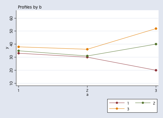
Graph of Cell Means from the 3x3 Factorial Example
Tests of Simple Main Effects
Source             SS  df       MS       F
A              190.00   2    95.00    1.52   n.s.
B             1543.33   2   771.67   12.35   sig.
A*B           1236.67   4   309.17    4.95   sig
  B at a1       63.33   2    31.67    0.51   n.s.
  B at a2      103.33   2    51.67    0.83   n.s.
  B at a3     2613.33   2  1306.67   20.91   sig.
Wcell         2250.00  36    62.50
Total         5220.00  44
Tests of Simple Main Effects in Stata
use http://www.philender.com/courses/data/crf33, clear

anova y a b a#b

                           Number of obs =      45     R-squared     =  0.5690
                           Root MSE      = 7.90569     Adj R-squared =  0.4732

                  Source |  Partial SS    df       MS           F     Prob > F
              -----------+----------------------------------------------------
                   Model |        2970     8      371.25       5.94     0.0001
                         |
                       a |         190     2          95       1.52     0.2324
                       b |  1543.33333     2  771.666667      12.35     0.0001
                     a#b |  1236.66667     4  309.166667       4.95     0.0028
                         |
                Residual |        2250    36        62.5
              -----------+----------------------------------------------------
                   Total |        5220    44  118.636364

sme b a

Test of b at a(1): F(2/36)  = .50666667
Test of b at a(2): F(2/36)  = .82666667
Test of b at a(3): F(2/36)  = 20.906667


Critical value of F for alpha = .05 using ...
--------------------------------------------------
Dunn's procedure              = 4.0941238
Marascuilo & Levin            = 4.5974255
per family error rate         = 4.5974255
simultaneous test procedure   = 6.5295994

anovalator b a, simple fratio

anovalator test of simple main effects for b at(a=1)
chi2(2) = 1.0133333   p-value = .60250057
scaled as F-ratio = .50666667

anovalator test of simple main effects for b at(a=2)
chi2(2) = 1.6533333   p-value = .43750521
scaled as F-ratio = .82666667

anovalator test of simple main effects for b at(a=3)
chi2(2) = 41.813333   p-value = 8.324e-10
scaled as F-ratio = 20.906667
Follow Up with Pairwise Comparisons at a3
tkcomp b if a==3

Tukey-Kramer pairwise comparisons for variable b
studentized range critical value(.05, 3, 36) = 3.4569115

                                      mean
grp vs grp       group means          dif     TK-test
-------------------------------------------------------
  1 vs   2    20.0000    40.0000     20.0000   5.6569*
  1 vs   3    20.0000    52.0000     32.0000   9.0510*
  2 vs   3    40.0000    52.0000     12.0000   3.3941

anovalator b, pair at(a=3) fratio

Adjusted predictions                              Number of obs   =         45

Expression   : Linear prediction, predict()
at           : a               =           3
               b                             (asbalanced)

------------------------------------------------------------------------------
             |            Delta-method
             |     Margin   Std. Err.      z    P>|z|     [95% Conf. Interval]
-------------+----------------------------------------------------------------
           b |
          1  |         20   3.535534     5.66   0.000     13.07048    26.92952
          2  |         40   3.535534    11.31   0.000     33.07048    46.92952
          3  |         52   3.535534    14.71   0.000     45.07048    58.92952
------------------------------------------------------------------------------

anovalator pairwise comparisons for b at(a=3)

Comparison          Coef.   Std. Err.      z    P>|z|     [95% Conf. Interval]
1 vs 2                -20          5       -4   0.000        -29.8       -10.2
1 vs 3                -32          5     -6.4   0.000        -41.8       -22.2
2 vs 3                -12          5     -2.4   0.016        -21.8        -2.2
Regression using anovalator
regress y a##b

      Source |       SS       df       MS              Number of obs =      45
-------------+------------------------------           F(  8,    36) =    5.94
       Model |        2970     8      371.25           Prob > F      =  0.0001
    Residual |        2250    36        62.5           R-squared     =  0.5690
-------------+------------------------------           Adj R-squared =  0.4732
       Total |        5220    44  118.636364           Root MSE      =  7.9057

------------------------------------------------------------------------------
           y |      Coef.   Std. Err.      t    P>|t|     [95% Conf. Interval]
-------------+----------------------------------------------------------------
           a |
          2  |         -3          5    -0.60   0.552    -13.14047     7.14047
          3  |        -13          5    -2.60   0.013    -23.14047    -2.85953
             |
           b |
          2  |          2          5     0.40   0.692     -8.14047    12.14047
          3  |          5          5     1.00   0.324     -5.14047    15.14047
             |
         a#b |
        2 2  |         -1   7.071068    -0.14   0.888    -15.34079    13.34079
        2 3  |          1   7.071068     0.14   0.888    -13.34079    15.34079
        3 2  |         18   7.071068     2.55   0.015      3.65921    32.34079
        3 3  |         27   7.071068     3.82   0.001     12.65921    41.34079
             |
       _cons |         33   3.535534     9.33   0.000      25.8296     40.1704
------------------------------------------------------------------------------


anovalator b a, main 2way fratio

anovalator main-effect for b
chi2(2) = 24.693333   p-value = 4.344e-06
scaled as F-ratio = 12.346667

anovalator main-effect for a
chi2(2) = 3.04   p-value = .21871189
scaled as F-ratio = 1.52

anovalator two-way interaction for b#a
chi2(4) = 19.786667   p-value = .00055023
scaled as F-ratio = 4.9466667

anovalator b a, simple fratio

anovalator test of simple main effects for b at(a=1)
chi2(2) = 1.0133333   p-value = .60250057
scaled as F-ratio = .50666667

anovalator test of simple main effects for b at(a=2)
chi2(2) = 1.6533333   p-value = .43750521
scaled as F-ratio = .82666667

anovalator test of simple main effects for b at(a=3)
chi2(2) = 41.813333   p-value = 8.324e-10
scaled as F-ratio = 20.906667
Consider the Following Plot of Cell Means
Would you need to do tests of simple main effects?
Would you need to follow up tests of simple main effects with pairwise comparisons?
Pooling
Philosophies on Pooling
Pooling
Simplified Pooling Example
Step 1: Without Pooling
Source    SS    df      MS         F
A         45     3   15.00     1.875    p>.05
B         72     4   18.00     2.250    p>.05
A*B        5    12     .42       <1     n.s.
Wcell    800   100    8.00
Total    922   119


Step 2: With Pooling
Source    SS    df      MS         F
A         45     3   15.00      2.11    p>.05
B         72     4   18.00      2.50    p<=.05
Error    805   112    7.19
Total    922   119
A More Complex Example of Pooling
Step 1: Without Pooling
Source
A
B
C
A*B
A*C
B*C
A*B*C
Wcell
Total
Step 2: Pool Highest Order Interaction
Source
A
B
C
A*B
A*C
B*C
Error = Wcell + A*B*C
Total
Step 3: Pool All Interactions
Source
A
B
C
Error = Wcell + A*B*C + A*B + A*C + B*C
Total
Pooling in Stata
Pooling in Stata can be accomplished simply leaving the appropriate interactions terms out of the anova command.
anova y a b c a#b a#c b#c a#b#c   /* no pooling */

anova y a b c a#b a#c b#c         /* pool a*b*c */

anova y a b c                     /* pool a*b a*c b*c a*b*c */
Interaction Example in a 3 Factor Model
use http://www.philender.com/courses/data/threeway, clear

anova y a##b##c


                           Number of obs =      24     R-squared     =  0.9689
                           Root MSE      =  1.1547     Adj R-squared =  0.9403

                  Source |  Partial SS    df       MS           F     Prob > F
              -----------+----------------------------------------------------
                   Model |  497.833333    11  45.2575758      33.94     0.0000
                         |
                       a |         150     1         150     112.50     0.0000
                       b |  .666666667     1  .666666667       0.50     0.4930
                     a#b |  160.166667     1  160.166667     120.13     0.0000
                       c |  127.583333     2  63.7916667      47.84     0.0000
                     a#c |       18.25     2       9.125       6.84     0.0104
                     b#c |  22.5833333     2  11.2916667       8.47     0.0051
                   a#b#c |  18.5833333     2  9.29166667       6.97     0.0098
                         |
                Residual |          16    12  1.33333333
              -----------+----------------------------------------------------
                   Total |  513.833333    23  22.3405797


anovalator b c, 2way at(a=1) fratio

anovalator two-way interaction for b#c at(a=1)
chi2(2) = 30.5   p-value = 2.382e-07
scaled as F-ratio = 15.25

anovalator b c, 2way at(a=2) fratio

anovalator two-way interaction for b#c at(a=2)
chi2(2) = .375   p-value = .82902912
scaled as F-ratio = .1875

anovalator c, main at(a=1 b=1) fratio

anovalator main-effect for c at(a=1 b=1)
chi2(2) = 48   p-value = 3.775e-11
scaled as F-ratio = 24

anovalator c, main at(a=1 b=2) fratio

anovalator main-effect for c at(a=1 b=2)
chi2(2) = 1   p-value = .60653066
scaled as F-ratio = .5

anovalator c, pairwise at(a=1 b=1) fratio

Adjusted predictions                              Number of obs   =         24

Expression   : Linear prediction, predict()
at           : a               =           1
               b               =           1
               c                             (asbalanced)

------------------------------------------------------------------------------
             |            Delta-method
             |     Margin   Std. Err.      z    P>|z|     [95% Conf. Interval]
-------------+----------------------------------------------------------------
           c |
          1  |         11   .8164966    13.47   0.000     9.399696     12.6003
          2  |         15   .8164966    18.37   0.000      13.3997     16.6003
          3  |         19   .8164966    23.27   0.000      17.3997     20.6003
------------------------------------------------------------------------------

anovalator pairwise comparisons for c at(a=1 b=1)

Comparison          Coef.   Std. Err.      z    P>|z|     [95% Conf. Interval]
1 vs 2                 -4     1.1547    -3.46   0.001    -6.263213   -1.736787
1 vs 3                 -8     1.1547    -6.93   0.000    -10.26321   -5.736787
2 vs 3                 -4     1.1547    -3.46   0.001    -6.263213   -1.736787

tkcomp c if a==1 & b==1

Tukey-Kramer pairwise comparisons for variable c
studentized range critical value(.05, 3, 12) = 3.772768

                                      mean
grp vs grp       group means          dif     TK-test
-------------------------------------------------------
  1 vs   2    11.0000    15.0000      4.0000   4.8990*
  1 vs   3    11.0000    19.0000      8.0000   9.7980*
  2 vs   3    15.0000    19.0000      4.0000   4.8990*
anovalator b c, 2way at(a=1) fratio
anovalator two-way interaction for b#c at(a=1)
chi2(2) = 30.5 p-value = 2.382e-07
scaled as F-ratio = 15.25
anovalator b c, 2way at(a=2) fratio
anovalator two-way interaction for b#c at(a=2)
chi2(2) = .375 p-value = .82902912
scaled as F-ratio = .1875
anovalator c, main at(a=1 b=1) fratio
anovalator main-effect for c at(a=1 b=1)
chi2(2) = 48 p-value = 3.775e-11
scaled as F-ratio = 24
anovalator c, main at(a=1 b=2) fratio
anovalator main-effect for c at(a=1 b=2)
chi2(2) = 1 p-value = .60653066
scaled as F-ratio = .5
anovalator c, pairwise at(a=1 b=1) fratio
Adjusted predictions Number of obs = 24
Expression : Linear prediction, predict()
at : a = 1
b = 1
c (asbalanced)
------------------------------------------------------------------------------
| Delta-method
| Margin Std. Err. z P>|z| [95% Conf. Interval]
-------------+----------------------------------------------------------------
c |
1 | 11 .8164966 13.47 0.000 9.399696 12.6003
2 | 15 .8164966 18.37 0.000 13.3997 16.6003
3 | 19 .8164966 23.27 0.000 17.3997 20.6003
------------------------------------------------------------------------------
anovalator pairwise comparisons for c at(a=1 b=1)
Comparison Coef. Std. Err. z P>|z| [95% Conf. Interval]
1 vs 2 -4 1.1547 -3.46 0.001 -6.263213 -1.736787
1 vs 3 -8 1.1547 -6.93 0.000 -10.26321 -5.736787
2 vs 3 -4 1.1547 -3.46 0.001 -6.263213 -1.736787
tkcomp c if a==1 & b==1
Tukey-Kramer pairwise comparisons for variable c
studentized range critical value(.05, 3, 12) = 3.772768
mean
grp vs grp group means dif TK-test
-------------------------------------------------------
1 vs 2 11.0000 15.0000 4.0000 4.8990*
1 vs 3 11.0000 19.0000 8.0000 9.7980*
2 vs 3 15.0000 19.0000 4.0000 4.8990*
Linear Statistical Models Course
Phil Ender, 17sep10, 12Feb98