Completely Randomized Model

Linear Statistical Models

Completely Randomized Design

Updated for Stata 11

CR-p -- Fixed Effects Model

AKA - One-way Analysis of variance, One-way ANOVA.

Schematic with Example Data

Level a1 a2 a3 a4 Total
4
6
3
3
1
3
2
2 4
5
4
3
2
3
4
3 5
6
5
4
3
4
3
4 3
5
6
5
6
7
8
10
Mean 3.0 3.5 4.25 6.25 4.25
sd 1.51 0.93 1.04 2.12 1.88

Or in abbreviated form:

Level a1 a2 a3 a4 Total
S₁
n=8 S₂
n=8 S₃
n=8 S₄
n=8
Mean 3.0 3.5 4.25 6.25 4.25
sd 1.51 0.93 1.04 2.12 1.88

Where each S_j is an independent randomly assigned group of subjects.

Linear Model

Y_ij = μ + α_j + ε_i(j)

The prediction model is

Y'_j = μ + α_j

where,

Y_ij is the score for the ith observation in the jth treatment level
Y'_j is the predicted value for the jth treatment level and is equal to the mean of the group
μ is the overall population mean (grand mean)
α_j is the effect of A treatment level j which is equal to μ_j - μ and is subject to the restriction that Σα_j = 0 over j
ε_i(j) is the error effect associated with Y_ij and is equal to Y_ij - μ - α_j . The error effect is a random variable that is distributed NID(0,s²_ε)

Hypotheses

Hypotheses are stated in terms of the treatment effect, α_j

H₀: α_j = 0 for all j
H₁: α_j ≠ 0 for some j

Assumptions

1. The linear model reflects all sources of variation.
2. The experiment contains all the treatment levels of interest.
3. The ε_i(j) are independent of each other.
4. The ε_i(j) are normally distributed.
5. The ε_i(j) have equal variance in the population.

Notes:
Assumptions 1 & 2 are concerned with model specification.
Because μ and α_j are constants, the following holds

ANOVA Summary Table

Source SS df MS F p-value

Between Groups 49.0 3 16.333 7.50 0.0008

Within Groups 61.0 28 2.179

Total 110.0 31

The ANOVA Summary Table may also look like this:

Source SS df MS F p-value

Treatment 49.0 3 16.333 7.50 0.0008

Error 61.0 28 2.179

Total 110.0 31

Table of the F-distribution

Between Groups = Treatment or use the variable name.

Within Groups = Error or Residual

Expected Mean Squares

Correctly Formed F-ratios

Table of Group Means and Variances

a1 a2 a3 a4
Mean 3.00 3.50 4.25 6.25
Variance 2.29 0.86 1.07 4.50

Std Dev 1.51 0.93 1.04 2.12

A Measure of Strength of Association

Omega-squared (ω²) is the recommended measure of strength of association for fixed-effects analysis of variance models.

From the Example:

      49 - (3)2.179
ω² = ---------------  = 0.3785
       110 + 2.179

Approximately 38% of the variability of the dependent variable can be explained by the independent variable, that is, by the differences among the four levels of the categorical variable.

The following guidelines are suggested by Cohen (1989):

ω² = .01 is a small association
ω² = .06 is a medium association
ω² = .14 is a large association

By these guidelines the ω² = .38 is very large, but this is because the example an artificial classroom dataset.

In terms of the fhat index of effect size:

fhat = .10 is a small effect
fhat = .25 is a medium effect
fhat = .40 is a large effect

These are very rough guidelines.

Note: The fhat index of effect size should not be confused with Cohen's d index of effect size. The fhat index is derived directly form the ω².

Model for Orthogonal Coding

G  X1  X2  X3
1   1   1   1
2  -1   1   1
3   0  -2   1
4   0   0  -3

Stata Computer Example

input y grp x1 x2 x3
 4 1  1  1  1
 6 1  1  1  1
 3 1  1  1  1
 3 1  1  1  1
 1 1  1  1  1
 3 1  1  1  1
 2 1  1  1  1
 2 1  1  1  1
 4 2 -1  1  1
 5 2 -1  1  1
 4 2 -1  1  1
 3 2 -1  1  1
 2 2 -1  1  1
 3 2 -1  1  1
 4 2 -1  1  1
 3 2 -1  1  1
 5 3  0 -2  1
 6 3  0 -2  1
 5 3  0 -2  1
 4 3  0 -2  1
 3 3  0 -2  1
 4 3  0 -2  1
 3 3  0 -2  1
 4 3  0 -2  1
 3 4  0  0 -3
 5 4  0  0 -3
 6 4  0  0 -3
 5 4  0  0 -3
 6 4  0  0 -3
 7 4  0  0 -3
 8 4  0  0 -3
10 4  0  0 -3
end

tabstat y, by(grp) stat(n mean sd var)

Summary for variables: y
     by categories of: grp 

     grp |         N      mean        sd  variance
---------+----------------------------------------
       1 |         8         3  1.511858  2.285714
       2 |         8       3.5  .9258201  .8571429
       3 |         8      4.25  1.035098  1.071429
       4 |         8      6.25   2.12132       4.5
---------+----------------------------------------
   Total |        32      4.25  1.883716  3.548387
--------------------------------------------------

display 2.12132/.9258201

2.2912875

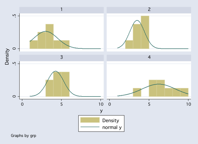
histogram y, by(grp) normal

robvar y, by(grp)   /* W0 is Levene's test of homoscedasticity */

            |            Summary of y
        grp |        Mean   Std. Dev.       Freq.
------------+------------------------------------
          1 |           3   1.5118579           8
          2 |         3.5    .9258201           8
          3 |        4.25   1.0350983           8
          4 |        6.25   2.1213203           8
------------+------------------------------------
      Total |        4.25   1.8837163          32

W0  = 1.292876   df(3, 28)     Pr > F = .29625408

W50 = 1.037037   df(3, 28)     Pr > F = .39138742

W10 = 1.292876   df(3, 28)     Pr > F = .29625408

anova y grp 

                           Number of obs =      32     R-squared     =  0.4455
                           Root MSE      =   1.476     Adj R-squared =  0.3860

                  Source |  Partial SS    df       MS           F     Prob > F
              -----------+----------------------------------------------------
                   Model |       49.00     3  16.3333333       7.50     0.0008
                         |
                     grp |       49.00     3  16.3333333       7.50     0.0008
                         |
                Residual |       61.00    28  2.17857143   
              -----------+----------------------------------------------------
                   Total |      110.00    31   3.5483871 

/* user written program -- findit effectsize */

effectsize grp  

 anova effect size for grp with dep var = y

total variance accounted for
omega2         = .37854187
eta2           = .44545455
Cohen's f      = .78046067

partial variance accounted for
partial omega2 = .37854187
partial eta2   = .44545455

/* Tukey-Kramer pairwise comparisons */
/* user written program -- findit tkcomp */

tkcomp grp  

Tukey-Kramer pairwise comparisons for variable grp
studentized range critical value(.05, 4, 28) = 3.8613586

                                      mean 
grp vs grp       group means          dif     TK-test
-------------------------------------------------------
  1 vs   2     3.0000     3.5000      0.5000   0.9581 
  1 vs   3     3.0000     4.2500      1.2500   2.3954 
  1 vs   4     3.0000     6.2500      3.2500   6.2279*
  2 vs   3     3.5000     4.2500      0.7500   1.4372 
  2 vs   4     3.5000     6.2500      2.7500   5.2698*
  3 vs   4     4.2500     6.2500      2.0000   3.8326 



oneway y grp, noanova sidak bonferroni scheffe

                            Comparison of y by grp
                                (Bonferroni)
Row Mean-|
Col Mean |          1          2          3
---------+---------------------------------
       2 |         .5
         |      1.000
         |
       3 |       1.25        .75
         |      0.608      1.000
         |
       4 |       3.25       2.75          2
         |      0.001      0.005      0.068

                            Comparison of y by grp
                                  (Scheffe)
Row Mean-|
Col Mean |          1          2          3
---------+---------------------------------
       2 |         .5
         |      0.927
         |
       3 |       1.25        .75
         |      0.427      0.794
         |
       4 |       3.25       2.75          2
         |      0.002      0.009      0.085

                            Comparison of y by grp
                                   (Sidak)
Row Mean-|
Col Mean |          1          2          3
---------+---------------------------------
       2 |         .5
         |      0.985
         |
       3 |       1.25        .75
         |      0.474      0.900
         |
       4 |       3.25       2.75          2
         |      0.001      0.005      0.066
       
/* regression with orthogonal coding */

regress y x1 x2 x3

      Source |       SS       df       MS              Number of obs =      32
-------------+------------------------------           F(  3,    28) =    7.50
       Model |       49.00     3  16.3333333           Prob > F      =  0.0008
    Residual |       61.00    28  2.17857143           R-squared     =  0.4455
-------------+------------------------------           Adj R-squared =  0.3860
       Total |      110.00    31   3.5483871           Root MSE      =   1.476

------------------------------------------------------------------------------
           y |      Coef.   Std. Err.      t    P>|t|     [95% Conf. Interval]
-------------+----------------------------------------------------------------
          x1 |       -.25   .3689996    -0.68   0.504    -1.005861    .5058614
          x2 |  -.3333333    .213042    -1.56   0.129    -.7697301    .1030635
          x3 |  -.6666667   .1506435    -4.43   0.000    -.9752458   -.3580875
       _cons |       4.25   .2609221    16.29   0.000     3.715525    4.784475
------------------------------------------------------------------------------ 

/* regression with dummy coding */

regress y i.grp


      Source |       SS       df       MS              Number of obs =      32
-------------+------------------------------           F(  3,    28) =    7.50
       Model |          49     3  16.3333333           Prob > F      =  0.0008
    Residual |          61    28  2.17857143           R-squared     =  0.4455
-------------+------------------------------           Adj R-squared =  0.3860
       Total |         110    31   3.5483871           Root MSE      =   1.476

------------------------------------------------------------------------------
           y |      Coef.   Std. Err.      t    P>|t|     [95% Conf. Interval]
-------------+----------------------------------------------------------------
         grp |
          2  |         .5   .7379992     0.68   0.504    -1.011723    2.011723
          3  |       1.25   .7379992     1.69   0.101    -.2617229    2.761723
          4  |       3.25   .7379992     4.40   0.000     1.738277    4.761723
             |
       _cons |          3   .5218443     5.75   0.000      1.93105     4.06895
------------------------------------------------------------------------------

/* cell means using margins command */

margins grp

Adjusted predictions                              Number of obs   =         32
Model VCE    : OLS

Expression   : Linear prediction, predict()

------------------------------------------------------------------------------
             |            Delta-method
             |     Margin   Std. Err.      z    P>|z|     [95% Conf. Interval]
-------------+----------------------------------------------------------------
         grp |
          1  |          3   .5218443     5.75   0.000     1.977204    4.022796
          2  |        3.5   .5218443     6.71   0.000     2.477204    4.522796
          3  |       4.25   .5218443     8.14   0.000     3.227204    5.272796
          4  |       6.25   .5218443    11.98   0.000     5.227204    7.272796
------------------------------------------------------------------------------

Some Formulas

Recall the linear model,

The grand mean is the general level of scores,

The treatment effect is the elevation or depression of scores due to the jth treatment,

The error effect is unique to subject i in treatment level j,

The above implies,

From the prediction model (way above),

Partitioning Sums of Squares

Linear Statistical Models Course

Phil Ender, 17sep10, 11apr06, 12Feb98

Level	a1	a2	a3	a4	Total
	4 6 3 3 1 3 2 2	4 5 4 3 2 3 4 3	5 6 5 4 3 4 3 4	3 5 6 5 6 7 8 10
Mean	3.0	3.5	4.25	6.25	4.25
sd	1.51	0.93	1.04	2.12	1.88

Level	a1	a2	a3	a4	Total
	S₁ n=8	S₂ n=8	S₃ n=8	S₄ n=8
Mean	3.0	3.5	4.25	6.25	4.25
sd	1.51	0.93	1.04	2.12	1.88

Source	SS	df	MS	F	p-value
Between Groups	49.0	3	16.333	7.50	0.0008
Within Groups	61.0	28	2.179
Total	110.0	31

Source	SS	df	MS	F	p-value
Treatment	49.0	3	16.333	7.50	0.0008
Error	61.0	28	2.179
Total	110.0	31

	a1	a2	a3	a4
Mean	3.00	3.50	4.25	6.25
Variance	2.29	0.86	1.07	4.50
Std Dev	1.51	0.93	1.04	2.12