Testing Variances

Introduction to Research Design and Statistics

Testing Variances

Warning

The single-sample chi-square test, the two-sample F-test, and the F-max test are all extremely sensitive to nonnormality. It can be difficult in practice to tell whether significant test values are due to heterogeneity of variance or to the fact that the populations are not normal. Users are cautioned against the routine use of the F-test or F-max test for verifying homogeneity of variance. Inspecting distributions graphically is a better practice.

Testing a Single Variance

The test of a single variance is performed using a chi-square test and the chi-square distribution.

χ² = (n - 1)s²/σ₀²,

where σ₀² is the hypothesized population variance.

The degrees of freedom, df = n - 1.

Use the table of the Chi-Square Distribution.

Example

Suppose a sample 30 observations is drawn from a population with σ₀² = 4.55 (σ₀ = 2.13). The sample variance, s² = 6.7 (s = 2.59). Test the hypothesis that the sample comes from a population with a variance greater than 4.55

₀

₁

df = n - 1 = 30 - 1 = 29

Critical value of chi-square = 42.56 at alpha = .05.

Compute chi-square:
chi-square = (30 - 1)6.7/4.55 = 42.7 Decision: Reject H₀

Conclusion: The sample of 30 observations comes from a distribution with a variance greater than 4.55.

Stata Examples

sdtesti 30 . 2.59 2.13

One-sample test of variance

------------------------------------------------------------------------------
         |     Obs        Mean    Std. Err.   Std. Dev.   [95% Conf. Interval]
---------+--------------------------------------------------------------------
       x |      30           .    .4728671        2.59           .           .
------------------------------------------------------------------------------

                              Ho: sd(x) = 2.13 
                              chi2(29) = 42.878

   Ha: sd(x) < 2.13           Ha: sd(x) ~= 2.13          Ha: sd(x) > 2.13
   P < chi2 = 0.9533        2*(P > chi2) = 0.0934        P > chi2 = 0.0467
 
use http://www.philender.com/courses/data/hsb2, clear
 
sdtest math=10.2

One-sample test of variance

------------------------------------------------------------------------------
Variable |     Obs        Mean    Std. Err.   Std. Dev.   [95% Conf. Interval]
---------+--------------------------------------------------------------------
    math |     200      52.645    .6624493    9.368448    51.33868    53.95132
------------------------------------------------------------------------------

                            Ho: sd(math) = 10.2 
                             chi2(199) = 167.876

  Ha: sd(math) < 10.2       Ha: sd(math) ~= 10.2        Ha: sd(math) > 10.2
   P < chi2 = 0.0531        2*(P < chi2) = 0.1061        P > chi2 = 0.9469

F distribution

Use the table of the F Distribution with numerator and denominator degrees of freedom.

Test Two Variances

It is possible to test any two variances from independent samples.

with degrees of freedom = n₁ - 1 and n₂ - 1.

Example

A math test is given in two classrooms. In the first classroom (21 students) the mean was 84.3 and the variance was 16.8. In the second classroom (16 students) the mean was 83.7 with a variance of 42.6. Are the two classroom variances different?

Compute the F-test: F = s²_larger/s²_smaller = 42.6/16.8 = 2.54.

Compute degrees of freedom: df = 15 and 20.

The critical value of F at alpha = 0.05 is 2.20.

Decision: Reject H₀, the variances are significantly different.

Example Using Stata

display sqrt(16.8)
4.0987803
 
display sqrt(42.6)
6.5268675
 
sdtesti 21 84.3 4.1 16 83.7 6.53

Variance ratio test

------------------------------------------------------------------------------
         |     Obs        Mean    Std. Err.   Std. Dev.   [95% Conf. Interval]
---------+--------------------------------------------------------------------
       x |      21        84.3    .8946933         4.1     82.4337     86.1663
       y |      16        83.7      1.6325        6.53    80.22041    87.17959
---------+--------------------------------------------------------------------
combined |      37    84.04054    .8573489     5.21505    82.30176    85.77932
------------------------------------------------------------------------------

                             Ho: sd(x) = sd(y) 

              F(20,15) observed   = F_obs           =    0.394
              F(20,15) lower tail = F_L   = F_obs   =    0.394
              F(20,15) upper tail = F_U   = 1/F_obs =    2.537

   Ha: sd(x) < sd(y)         Ha: sd(x) ~= sd(y)          Ha: sd(x) > sd(y)
  P < F_obs = 0.0267     P < F_L + P > F_U = 0.0622     P > F_obs = 0.9733

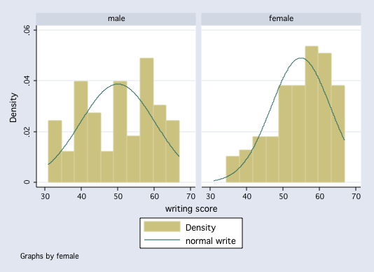
Stata Example

This example illustrates how the F-ratio for equal variances can abe misleading.

use http://www.gseis.ucla.edu/courses/data/hsb2
 
sdtest write, by(female)

Variance ratio test

------------------------------------------------------------------------------
   Group |     Obs        Mean    Std. Err.   Std. Dev.   [95% Conf. Interval]
---------+--------------------------------------------------------------------
    male |      91    50.12088    1.080274    10.30516    47.97473    52.26703
  female |     109    54.99083    .7790686    8.133715    53.44658    56.53507
---------+--------------------------------------------------------------------
combined |     200      52.775    .6702372    9.478586    51.45332    54.09668
------------------------------------------------------------------------------

                         Ho: sd(male) = sd(female) 

              F(90,108) observed   = F_obs           =    1.605
              F(90,108) lower tail = F_L   = 1/F_obs =    0.623
              F(90,108) upper tail = F_U   = F_obs   =    1.605

   Ha: sd(1) < sd(2)         Ha: sd(1) ~= sd(2)          Ha: sd(1) > sd(2)
  P < F_obs = 0.9906     P < F_L + P > F_U = 0.0199     P > F_obs = 0.0094

histogram write, by(female) normal bin(10)

F-max Test

The Fmax test is used to test homogeneity of variance in one-way analysis of variance (ANOVA).

with degrees of freedom = k (number of groups) and n - 1 (number in each group).

You need to use the Table of the F-max Distribution.

Example

Thirty-two subjects are randomly assigned to one of four groups. One control group and three groups with progressively increasing amount of reward. The means and variances of the three groups are: G1 = 2.75 & 1.714, G2 = 3.5 & 0.857, G2 = 6.25 & 1.071, and G4 = 9 & 2.214.

Compute the F-test: F = s²_largest/s²_smallest = 2.214/0.857 = 2.58.

Calculate degrees of freedom: number of groups = 4, number in each group = 8,
df = 4 & 7.

Critical value of F-max at alpha = 0.05 is 8.44.

Decision: Fail to reject H₀, variances are not significantly different, there is homogeneity of variance.

Test Pearson Correlation Using F

Here is a way to test whether a Pearson Correlation Coefficient is significantly different from zero.

with degrees of freedom = 1 and n - 2.

Example

The correlation between physical punishment and aggression was .32 in a sample of 62 children. Is this correlation significant?

Compute F: F = r²/((1-r²)/(n-2)) = .1024/((1-.1024)/(62-2)) = 6.84.

Compute degrees of freedom: df = 1 and n - 2 = 60.

Critical value of F at alpha = 0.05 is 4.00.

Decision: Reject H₀, correlation is statistically significant.

Intro Home Page

Phil Ender, 11Nov00