input id x
13 34
17 21
14 25
 9 33
18 40
12 33
 4 44
11 41
17 21
end

sort id

list

     +---------+
     | id    x |
     |---------|
  1. | 13   34 |
  2. | 17   21 |
  3. | 14   25 |
  4. |  9   33 |
  5. | 18   40 |
     |---------|
  6. | 12   33 |
  7. |  4   44 |
  8. | 11   41 |
  9. | 17   21 |
     +---------+
Part 2: Descriptive statistics and exploratory data analysis
use http://www.philender.com/courses/data/hsb2, clear
describe
Contains data from http://www.gseis.ucla.edu/courses/data/hsb2.dta
obs: 200 highschool and beyond (200
cases)
vars: 11 21 Jun 2000 08:54
size: 9,600 (98.9% of memory free)
-------------------------------------------------------------------------------
storage display value
variable name type format label variable label
-------------------------------------------------------------------------------
id float %9.0g
female float %9.0g fl
race float %12.0g rl
ses float %9.0g sl
schtyp float %9.0g scl type of school
prog float %9.0g sel type of program
read float %9.0g reading score
write float %9.0g writing score
math float %9.0g math score
science float %9.0g science score
socst float %9.0g social studies score
-------------------------------------------------------------------------------
list
list
Observation 1
id 70 female male race white
ses low schtyp public prog general
read 57 write 52 math 41
science 47 socst 57
Observation 2
id 121 female female race white
ses middle schtyp public prog vocation
read 68 write 59 math 53
science 63 socst 61
Observation 3
id 86 female male race white
ses high schtyp public prog general
read 44 write 33 math 54
science 58 socst 31
Observation 4
id 141 female male race white
ses high schtyp public prog vocation
read 63 write 44 math 47
science 53 socst 56
Observation 5
id 172 female male race white
ses middle schtyp public prog academic
read 47 write 52 math 57
science 53 socst 61
...
list id female race ses prog read in 1/20
+--------------------------------------------------------+
| id female race ses prog read |
|--------------------------------------------------------|
1. | 70 male white low general 57 |
2. | 121 female white middle vocation 68 |
3. | 86 male white high general 44 |
4. | 141 male white high vocation 63 |
5. | 172 male white middle academic 47 |
|--------------------------------------------------------|
6. | 113 male white middle academic 44 |
7. | 50 male african-amer middle general 50 |
8. | 11 male hispanic middle academic 34 |
9. | 84 male white middle general 63 |
10. | 48 male african-amer middle academic 57 |
|--------------------------------------------------------|
11. | 75 male white middle vocation 60 |
12. | 60 male white middle academic 57 |
13. | 95 male white high academic 73 |
14. | 104 male white high academic 54 |
15. | 38 male african-amer low academic 45 |
|--------------------------------------------------------|
16. | 115 male white low general 42 |
17. | 76 male white high academic 47 |
18. | 195 male white middle general 57 |
19. | 114 male white high academic 68 |
20. | 85 male white middle general 55 |
+--------------------------------------------------------+
list id female race ses prog read in 1/20, clean
id female race ses prog read
1. 70 male white low general 57
2. 121 female white middle vocation 68
3. 86 male white high general 44
4. 141 male white high vocation 63
5. 172 male white middle academic 47
6. 113 male white middle academic 44
7. 50 male african-amer middle general 50
8. 11 male hispanic middle academic 34
9. 84 male white middle general 63
10. 48 male african-amer middle academic 57
11. 75 male white middle vocation 60
12. 60 male white middle academic 57
13. 95 male white high academic 73
14. 104 male white high academic 54
15. 38 male african-amer low academic 45
16. 115 male white low general 42
17. 76 male white high academic 47
18. 195 male white middle general 57
19. 114 male white high academic 68
20. 85 male white middle general 55
list id female race ses prog read in 1/20, clean nolabel
id female race ses prog read
1. 70 0 4 1 1 57
2. 121 1 4 2 3 68
3. 86 0 4 3 1 44
4. 141 0 4 3 3 63
5. 172 0 4 2 2 47
6. 113 0 4 2 2 44
7. 50 0 3 2 1 50
8. 11 0 1 2 2 34
9. 84 0 4 2 1 63
10. 48 0 3 2 2 57
11. 75 0 4 2 3 60
12. 60 0 4 2 2 57
13. 95 0 4 3 2 73
14. 104 0 4 3 2 54
15. 38 0 3 1 2 45
16. 115 0 4 1 1 42
17. 76 0 4 3 2 47
18. 195 0 4 2 1 57
19. 114 0 4 3 2 68
20. 85 0 4 2 1 55
summarize
Variable | Obs Mean Std. Dev. Min Max
-------------+-----------------------------------------------------
id | 200 100.5 57.87918 1 200
female | 200 .545 .4992205 0 1
race | 200 3.43 1.039472 1 4
ses | 200 2.055 .7242914 1 3
schtyp | 200 1.16 .367526 1 2
prog | 200 2.025 .6904772 1 3
read | 200 52.23 10.25294 28 76
write | 200 52.775 9.478586 31 67
math | 200 52.645 9.368448 33 75
science | 200 51.85 9.900891 26 74
socst | 200 52.405 10.73579 26 71
summarize write
Variable | Obs Mean Std. Dev. Min Max
-------------+-----------------------------------------------------
write | 200 52.775 9.478586 31 67
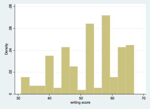
histogram write
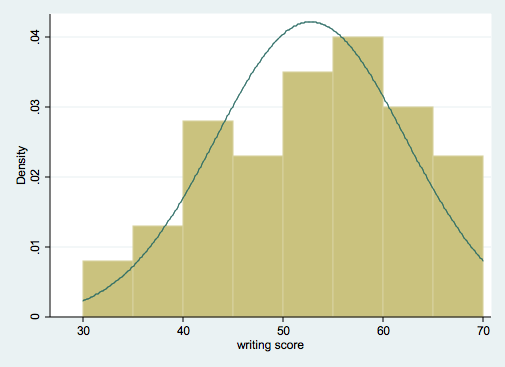
 histogram write, start(30) width(5) normal
 tabulate write
writing |
score | Freq. Percent Cum.
------------+-----------------------------------
31 | 4 2.00 2.00
33 | 4 2.00 4.00
35 | 2 1.00 5.00
36 | 2 1.00 6.00
37 | 3 1.50 7.50
38 | 1 0.50 8.00
39 | 5 2.50 10.50
40 | 3 1.50 12.00
41 | 10 5.00 17.00
42 | 2 1.00 18.00
43 | 1 0.50 18.50
44 | 12 6.00 24.50
45 | 1 0.50 25.00
46 | 9 4.50 29.50
47 | 2 1.00 30.50
49 | 11 5.50 36.00
50 | 2 1.00 37.00
52 | 15 7.50 44.50
53 | 1 0.50 45.00
54 | 17 8.50 53.50
55 | 3 1.50 55.00
57 | 12 6.00 61.00
59 | 25 12.50 73.50
60 | 4 2.00 75.50
61 | 4 2.00 77.50
62 | 18 9.00 86.50
63 | 4 2.00 88.50
65 | 16 8.00 96.50
67 | 7 3.50 100.00
------------+-----------------------------------
Total | 200 100.00
sort prog
by prog: summarize write
_______________________________________________________________________________
-> prog = general
Variable | Obs Mean Std. Dev. Min Max
-------------+-----------------------------------------------------
write | 45 51.33333 9.397775 31 67
_______________________________________________________________________________
-> prog = academic
Variable | Obs Mean Std. Dev. Min Max
-------------+-----------------------------------------------------
write | 105 56.25714 7.943343 33 67
_______________________________________________________________________________
-> prog = vocation
Variable | Obs Mean Std. Dev. Min Max
-------------+-----------------------------------------------------
write | 50 46.76 9.318754 31 67
summarize write, detail
writing score
-------------------------------------------------------------
Percentiles Smallest
1% 31 31
5% 35.5 31
10% 39 31 Obs 200
25% 45.5 31 Sum of Wgt. 200
50% 54 Mean 52.775
Largest Std. Dev. 9.478586
75% 60 67
90% 65 67 Variance 89.84359
95% 65 67 Skewness -.4784158
99% 67 67 Kurtosis 2.238527
stem write
Stem-and-leaf plot for write (writing score)
3* | 1111
3t | 3333
3f | 55
3s | 66777
3. | 899999
4* | 0001111111111
4t | 223
4f | 4444444444445
4s | 66666666677
4. | 99999999999
5* | 00
5t | 2222222222222223
5f | 44444444444444444555
5s | 777777777777
5. | 9999999999999999999999999
6* | 00001111
6t | 2222222222222222223333
6f | 5555555555555555
6s | 7777777
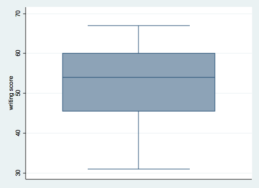
graph box write
tabulate write
writing |
score | Freq. Percent Cum.
------------+-----------------------------------
31 | 4 2.00 2.00
33 | 4 2.00 4.00
35 | 2 1.00 5.00
36 | 2 1.00 6.00
37 | 3 1.50 7.50
38 | 1 0.50 8.00
39 | 5 2.50 10.50
40 | 3 1.50 12.00
41 | 10 5.00 17.00
42 | 2 1.00 18.00
43 | 1 0.50 18.50
44 | 12 6.00 24.50
45 | 1 0.50 25.00
46 | 9 4.50 29.50
47 | 2 1.00 30.50
49 | 11 5.50 36.00
50 | 2 1.00 37.00
52 | 15 7.50 44.50
53 | 1 0.50 45.00
54 | 17 8.50 53.50
55 | 3 1.50 55.00
57 | 12 6.00 61.00
59 | 25 12.50 73.50
60 | 4 2.00 75.50
61 | 4 2.00 77.50
62 | 18 9.00 86.50
63 | 4 2.00 88.50
65 | 16 8.00 96.50
67 | 7 3.50 100.00
------------+-----------------------------------
Total | 200 100.00
sort prog
by prog: summarize write
_______________________________________________________________________________
-> prog = general
Variable | Obs Mean Std. Dev. Min Max
-------------+-----------------------------------------------------
write | 45 51.33333 9.397775 31 67
_______________________________________________________________________________
-> prog = academic
Variable | Obs Mean Std. Dev. Min Max
-------------+-----------------------------------------------------
write | 105 56.25714 7.943343 33 67
_______________________________________________________________________________
-> prog = vocation
Variable | Obs Mean Std. Dev. Min Max
-------------+-----------------------------------------------------
write | 50 46.76 9.318754 31 67
summarize write, detail
writing score
-------------------------------------------------------------
Percentiles Smallest
1% 31 31
5% 35.5 31
10% 39 31 Obs 200
25% 45.5 31 Sum of Wgt. 200
50% 54 Mean 52.775
Largest Std. Dev. 9.478586
75% 60 67
90% 65 67 Variance 89.84359
95% 65 67 Skewness -.4784158
99% 67 67 Kurtosis 2.238527
stem write
Stem-and-leaf plot for write (writing score)
3* | 1111
3t | 3333
3f | 55
3s | 66777
3. | 899999
4* | 0001111111111
4t | 223
4f | 4444444444445
4s | 66666666677
4. | 99999999999
5* | 00
5t | 2222222222222223
5f | 44444444444444444555
5s | 777777777777
5. | 9999999999999999999999999
6* | 00001111
6t | 2222222222222222223333
6f | 5555555555555555
6s | 7777777
graph box write
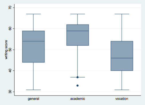
 graph box write, over(prog)
Part 3: Selecting Cases
Example 1use http://www.philender.com/courses/data/hsb2, clear
tabulate prog
type of |
program | Freq. Percent Cum.
------------+-----------------------------------
general | 45 22.50 22.50
academic | 105 52.50 75.00
vocation | 50 25.00 100.00
------------+-----------------------------------
Total | 200 100.00
summarize write if prog==1
Variable | Obs Mean Std. Dev. Min Max
-------------+--------------------------------------------------------
write | 45 51.33333 9.397775 31 67Example 2
You will have to clear and reload the data after this example.
keep if prog==1
(155 observations deleted)

tabulate prog

    type of |
    program |      Freq.     Percent        Cum.
------------+-----------------------------------
    general |         45      100.00      100.00
------------+-----------------------------------
      Total |         45      100.00

summarize write

    Variable |       Obs        Mean    Std. Dev.       Min        Max
-------------+--------------------------------------------------------
       write |        45    51.33333    9.397775         31         67
Part 4: Scatterplots, Correlation and Regression
use http://www.philender.com/courses/data/hsb2 scatter write readscatter write read, jitter(2)
scatter write read, jitter(2) msym(Oh)
twoway (scatter write read, jitter(2) msym(Oh))(lfit write read)
correlate write read math female (obs=200) | write read math female -------------+------------------------------------ write | 1.0000 read | 0.5968 1.0000 math | 0.6174 0.6623 1.0000 female | 0.2565 -0.0531 -0.0293 1.0000 sort female by female: correlate write read math ------------------------------------------------------------------------------- -> female = male (obs=91) | write read math -------------+--------------------------- write | 1.0000 read | 0.6485 1.0000 math | 0.6268 0.6085 1.0000 -------------------------------------------------------------------------------- -> female = female (obs=109) | write read math -------------+--------------------------- write | 1.0000 read | 0.6209 1.0000 math | 0.6749 0.7111 1.0000 regress write read Source | SS df MS Number of obs = 200 -------------+------------------------------ F( 1, 198) = 109.52 Model | 6367.42127 1 6367.42127 Prob > F = 0.0000 Residual | 11511.4537 198 58.1386552 R-squared = 0.3561 -------------+------------------------------ Adj R-squared = 0.3529 Total | 17878.875 199 89.843593 Root MSE = 7.6249 ------------------------------------------------------------------------------ write | Coef. Std. Err. t P>|t| [95% Conf. Interval] -------------+---------------------------------------------------------------- read | .5517051 .0527178 10.47 0.000 .4477445 .6556656 _cons | 23.95944 2.805744 8.54 0.000 18.42647 29.49242 ------------------------------------------------------------------------------ regress write read female Source | SS df MS Number of obs = 200 -------------+------------------------------ F( 2, 197) = 77.21 Model | 7856.32118 2 3928.16059 Prob > F = 0.0000 Residual | 10022.5538 197 50.8759077 R-squared = 0.4394 -------------+------------------------------ Adj R-squared = 0.4337 Total | 17878.875 199 89.843593 Root MSE = 7.1327 ------------------------------------------------------------------------------ write | Coef. Std. Err. t P>|t| [95% Conf. Interval] -------------+---------------------------------------------------------------- read | .5658869 .0493849 11.46 0.000 .468496 .6632778 female | 5.486894 1.014261 5.41 0.000 3.48669 7.487098 _cons | 20.22837 2.713756 7.45 0.000 14.87663 25.58011 ------------------------------------------------------------------------------
Part 5: Independent & Dependent t-tests
Example 1: Independent t-testuse http://www.philender.com/courses/data/hsb2, clear
ttest write, by(female)
Two-sample t test with equal variances
------------------------------------------------------------------------------
Group | Obs Mean Std. Err. Std. Dev. [95% Conf. Interval]
---------+--------------------------------------------------------------------
male | 91 50.12088 1.080274 10.30516 47.97473 52.26703
female | 109 54.99083 .7790686 8.133715 53.44658 56.53507
---------+--------------------------------------------------------------------
combined | 200 52.775 .6702372 9.478586 51.45332 54.09668
---------+--------------------------------------------------------------------
diff | -4.869947 1.304191 -7.441835 -2.298059
------------------------------------------------------------------------------
diff = mean(male) - mean(female) t = -3.7341
Ho: diff = 0 degrees of freedom = 198
Ha: diff < 0 Ha: diff != 0 Ha: diff > 0
Pr(T < t) = 0.0001 Pr(|T| > |t|) = 0.0002 Pr(T > t) = 0.9999Example 2: Dependent t-test
ttest write = read

Paired t test
------------------------------------------------------------------------------
Variable |     Obs        Mean    Std. Err.   Std. Dev.   [95% Conf. Interval]
---------+--------------------------------------------------------------------
   write |     200      52.775    .6702372    9.478586    51.45332    54.09668
    read |     200       52.23    .7249921    10.25294    50.80035    53.65965
---------+--------------------------------------------------------------------
    diff |     200        .545    .6283822    8.886666   -.6941424    1.784142
------------------------------------------------------------------------------
     mean(diff) = mean(write - read)                              t =   0.8673
 Ho: mean(diff) = 0                              degrees of freedom =      199

 Ha: mean(diff) < 0           Ha: mean(diff) != 0           Ha: mean(diff) > 0
 Pr(T < t) = 0.8066         Pr(|T| > |t|) = 0.3868          Pr(T > t) = 0.1934
Part 6: Contingency Tables/Crosstabulation
tabulate prog female, all

   type of |        female
   program |      male     female |     Total
-----------+----------------------+----------
   general |        21         24 |        45
  academic |        47         58 |       105
  vocation |        23         27 |        50
-----------+----------------------+----------
     Total |        91        109 |       200

          Pearson chi2(2) =   0.0528   Pr = 0.974
 likelihood-ratio chi2(2) =   0.0528   Pr = 0.974
               Cramér's V =   0.0162
                    gamma =   0.0066  ASE = 0.122
          Kendall's tau-b =   0.0036  ASE = 0.067
Part 7: Missing Data
How to Indicate Missing Data
In Stata, missing values are indicated by periods, ".".Example Dataset for Missing Data
Consider the hypothetical midterm and final exam test scores for 15 students in an elementary statistics course. The maximum is possible score is 50 points on each. There are two missing midterm scores and one missing final exam score. Look a the sample size for each variable and analysis.use http://www.philender.com/courses/data/missing, clear
describe
Contains data from missing.dta
obs: 15
vars: 2 14 Jul 2006 17:56
size: 180 (99.9% of memory free)
-------------------------------------------------------------------------------
storage display value
variable name type format label variable label
-------------------------------------------------------------------------------
mt float %9.0g
final float %9.0g
-------------------------------------------------------------------------------
Sorted by:
list, clean
mt final
1. 43 48
2. . 41
3. 41 44
4. 40 44
5. 38 43
6. 46 42
7. 41 40
8. 48 .
9. 42 45
10. 41 40
11. 43 46
12. . 45
13. 44 48
14. 39 42
15. 40 45
generate total = mt + final
(3 missing values generated)
list, clean
mt final total
1. 43 48 91
2. . 41 .
3. 41 44 85
4. 40 44 84
5. 38 43 81
6. 46 42 88
7. 41 40 81
8. 48 . .
9. 42 45 87
10. 41 40 81
11. 43 46 89
12. . 45 .
13. 44 48 92
14. 39 42 81
15. 40 45 85
summarize
Variable | Obs Mean Std. Dev. Min Max
-------------+--------------------------------------------------------
mt | 13 42 2.798809 38 48
final | 14 43.78571 2.607049 40 48
total | 12 85.41667 4.010403 81 92
correlate
(obs=12)
| mt final total
-------------+---------------------------
mt | 1.0000
final | 0.3263 1.0000
total | 0.7755 0.8498 1.0000
pwcorr, obs
| mt final total
-------------+---------------------------
mt | 1.0000
| 13
|
final | 0.3263 1.0000
| 12 14
|
total | 0.7755 0.8498 1.0000
| 12 12 12
Part 8: Logging Your Output
There will be many occassions wherre you will want to save all of the results from a Stata session. The output window only holds the last sewveral hundred lines and a session may include much more than that. To save your results you will need to create a log file of the session.
log using mylog1.log

[ a bunch of Stata commands ]

log close

type mylog1.log