Applied Categorical & Nonnormal Data Analysis
Correspondence Analysis
Correspondence analysis represents yet one more method for analyzing data in contingency
tables. Correspondence analysis was developed in France and is more commonly used in Europe than in
North America. Correspondence analysis is a descriptive/exploratory technique designed to analyze
two-way and multi-way tables containing measures of correspondence between the row and column
variables. The results produced by correspondence analysis provide information which is similar
to that produced by principal components or factor analysis. They allow one to explore the
structure of the categorical variables included in the table.
Correspondence analysis seeks to represent the relationships among the
categories of row and column variables with a smaller number of latent dimensions.
It produces a graphical representation of the relationships between the row and column categories
in the same space.
We will illustrate correspondence analysis using the ca command (new in Stata 9) with
the hsb2 dataset. In looking at the relationship
between race and ses there can be at most two dimensions. The maximum number
of dimensions is the minimum(R-1, C-1). Since ses has three categories, C-1 = 2.
In this example, as you will see, the first dimension accounts for about 98% of the
variability, so there is really only one dimension.
Some terminology: Mass is just the relative frequencies for each of the marginal categorites.
The total inertia is the chi-square value divided by N. It is partioned into parts for each of
the dimensions. We can write inertia as the weighted sum of the chi-square distance between each
profile and the mean profile.
Example 1
use http://www.gseis.ucla.edu/courses/data/hsb2,clear
tabulate race ses, chi2
| ses
race | low middle high | Total
-------------+---------------------------------+----------
hispanic | 9 11 4 | 24
asian | 3 5 3 | 11
african-amer | 11 6 3 | 20
white | 24 73 48 | 145
-------------+---------------------------------+----------
Total | 47 95 58 | 200
Pearson chi2(6) = 18.5160 Pr = 0.005
/* row profile */
tabulate race ses, row nofreq
| ses
race | low middle high | Total
-------------+---------------------------------+----------
hispanic | 37.50 45.83 16.67 | 100.00
asian | 27.27 45.45 27.27 | 100.00
african-amer | 55.00 30.00 15.00 | 100.00
white | 16.55 50.34 33.10 | 100.00
-------------+---------------------------------+----------
Total | 23.50 47.50 29.00 | 100.00
/* code to plot row profiles */
preserve
contract race ses
sort race
by race: gen rsum = sum(_freq)
by race: gen rpro = _freq/rsum[_N]
drop _freq rsum
reshape wide rpro, i(race) j(ses)
/* findit triplot */
triplot rpro1 rpro2 rpro3
 restore
ca race ses,
Correspondence analysis Number of obs = 200
Pearson chi2(6) = 18.52
Prob > chi2 = 0.0051
Total inertia = 0.0926
4 active rows Number of dim. = 2
3 active columns Expl. inertia (%) = 100.00
| singular principal cumul
Dimensions | values inertia chi2 percent percent
-------------+-----------------------------------------------------------
dim 1 | .3009322 .0905602 18.11 97.82 97.82
dim 2 | .0449396 .0020196 0.40 2.18 100.00
-------------+-----------------------------------------------------------
total | .0925798 18.52 100
Statistics for row and column categories in symmetric normalization
| overall | dimension_1 | dimension_2
Categories | mass quality inertia | coord sqcorr contrib | coord sqcorr contrib
-------------+---------------------------+---------------------------+---------------------------
race | | |
hispanic | 0.120 1.000 0.016 | 0.643 0.913 0.165 | 0.515 0.087 0.709
asian | 0.055 1.000 0.000 | 0.162 0.993 0.005 | -0.036 0.007 0.002
african-amer | 0.100 1.000 0.055 | 1.350 0.990 0.606 | -0.349 0.010 0.270
white | 0.725 1.000 0.020 | -0.305 0.998 0.224 | -0.034 0.002 0.019
-------------+---------------------------+---------------------------+---------------------------
ses | | |
low | 0.235 1.000 0.067 | 0.976 0.999 0.744 | -0.063 0.001 0.021
middle | 0.475 1.000 0.008 | -0.220 0.884 0.076 | 0.206 0.116 0.449
high | 0.290 1.000 0.017 | -0.431 0.938 0.179 | -0.287 0.062 0.531
-------------------------------------------------------------------------------------------------
restore
ca race ses,
Correspondence analysis Number of obs = 200
Pearson chi2(6) = 18.52
Prob > chi2 = 0.0051
Total inertia = 0.0926
4 active rows Number of dim. = 2
3 active columns Expl. inertia (%) = 100.00
| singular principal cumul
Dimensions | values inertia chi2 percent percent
-------------+-----------------------------------------------------------
dim 1 | .3009322 .0905602 18.11 97.82 97.82
dim 2 | .0449396 .0020196 0.40 2.18 100.00
-------------+-----------------------------------------------------------
total | .0925798 18.52 100
Statistics for row and column categories in symmetric normalization
| overall | dimension_1 | dimension_2
Categories | mass quality inertia | coord sqcorr contrib | coord sqcorr contrib
-------------+---------------------------+---------------------------+---------------------------
race | | |
hispanic | 0.120 1.000 0.016 | 0.643 0.913 0.165 | 0.515 0.087 0.709
asian | 0.055 1.000 0.000 | 0.162 0.993 0.005 | -0.036 0.007 0.002
african-amer | 0.100 1.000 0.055 | 1.350 0.990 0.606 | -0.349 0.010 0.270
white | 0.725 1.000 0.020 | -0.305 0.998 0.224 | -0.034 0.002 0.019
-------------+---------------------------+---------------------------+---------------------------
ses | | |
low | 0.235 1.000 0.067 | 0.976 0.999 0.744 | -0.063 0.001 0.021
middle | 0.475 1.000 0.008 | -0.220 0.884 0.076 | 0.206 0.116 0.449
high | 0.290 1.000 0.017 | -0.431 0.938 0.179 | -0.287 0.062 0.531
-------------------------------------------------------------------------------------------------
 /* for ethnic */
cabiplot , nocolumn origin
/* for ethnic */
cabiplot , nocolumn origin
 /* for ses */
cabiplot , norow origin
/* for ses */
cabiplot , norow origin
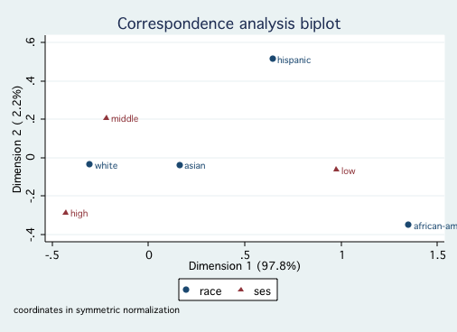
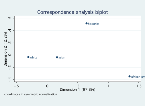
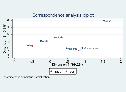
Since both race and ses reflect socioeconomic factors, it is not surprising that
they fall primarily onto a single dimension. Looking at the first graph shows that White and Asian
are close to one another on Dimension 1, followed by Hispanic and further away African-American.
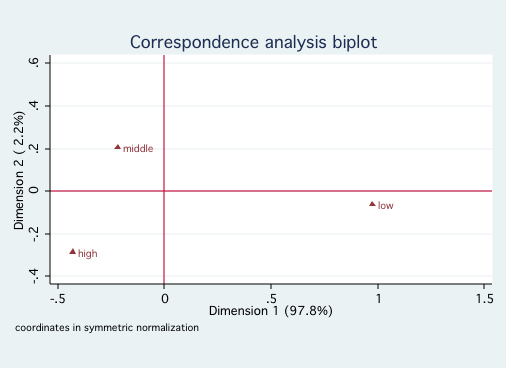
The second graph indicates that high and middle ses are close to one another with low ses much
further away. There is nothing in this analysis to contradict ones common sense interpretation of
these variables.
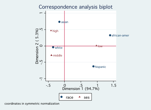
Example 2
Next, we will try the same correspondence analysis separately by gender with numeric
results suppressed.
quietly ca race ses if ~female

cabiplot , origin


quietly ca race ses if female

cabiplot , origin
quietly ca race ses if female
cabiplot , origin
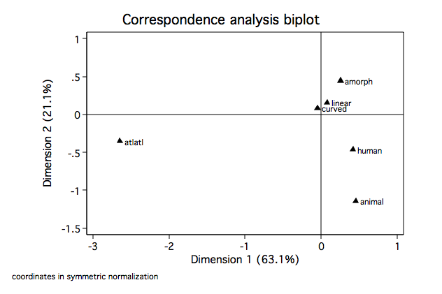
Example 3
This is an example from anthropology involving Native American petroglyphs from
eight different sites. We will be using the matrix version of the correspondence command,
camat. The petroglyphs are categorized into six different motifs:
linear, animal, atlatl, curved, human and amorph (for amorphouss).
The data form an 8x6 table giving the number of each motif located at each of
the eight sites (rows).
use http://www.philender.com/courses/data/petroglyph, clear

clist

        linear     animal     atlatl     curved      human     amorph
  1.        62         15          1         93          9         87
  2.       154         25        121        255         11         81
  3.        80         27          3        165          4         59
  4.        80         59          2        106         18         35
  5.       144         36          1        216         14        127
  6.        72         53          7        140         20         23
  7.       329        105         10        350         46        204
  8.        61         85         17        100          9         79
A quick look suggests that the atlatl motif has an unusual distribution in that
roughly 75% of the atlatl pictoglyphs were found at a single site, site 2. Let's
run the correspondence analysis and see what else we can find.
mkmat linear animal atlatl curved human amorph, mat(A)
mat rownames A = s1 s2 s3 s4 s5 s6 s7 s8
mat list A
A[8,6]
linear animal atlatl curved human amorph
s1 62 15 1 93 9 87
s2 154 25 121 255 11 81
s3 80 27 3 165 4 59
s4 80 59 2 106 18 35
s5 144 36 1 216 14 127
s6 72 53 7 140 20 23
s7 329 105 10 350 46 204
s8 61 85 17 100 9 79
camat A
Correspondence analysis Number of obs = 3800
Pearson chi2(35) = 702.36
Prob > chi2 = 0.0000
Total inertia = 0.1848
8 active rows Number of dim. = 2
6 active columns Expl. inertia (%) = 84.21
| singular principal cumul
Dimension | value inertia chi2 percent percent
------------+------------------------------------------------------------
dim 1 | .341633 .1167131 443.51 63.15 63.15
dim 2 | .1973312 .0389396 147.97 21.07 84.21
dim 3 | .1363464 .0185903 70.64 10.06 94.27
dim 4 | .0943349 .0088991 33.82 4.81 99.09
dim 5 | .0411102 .0016901 6.42 0.91 100.00
------------+------------------------------------------------------------
total | .1848322 702.36 100
Statistics for row and column categories in symmetric normalization
| overall | dimension_1
Categories | mass quality %inert | coord sqcorr contrib
-------------+---------------------------+---------------------------
rows | |
s1 | 0.070 0.704 0.067 | 0.338 0.222 0.023
s2 | 0.170 1.000 0.518 | -1.282 0.999 0.819
s3 | 0.089 0.300 0.041 | 0.171 0.118 0.008
s4 | 0.079 0.925 0.064 | 0.386 0.337 0.034
s5 | 0.142 0.964 0.056 | 0.291 0.393 0.035
s6 | 0.083 0.590 0.068 | 0.178 0.071 0.008
s7 | 0.275 0.684 0.069 | 0.288 0.614 0.067
s8 | 0.092 0.550 0.117 | 0.150 0.033 0.006
-------------+---------------------------+---------------------------
columns | |
linear | 0.258 0.259 0.038 | 0.079 0.080 0.005
animal | 0.107 0.956 0.199 | 0.457 0.207 0.065
atlatl | 0.043 0.992 0.563 | -2.648 0.982 0.875
curved | 0.375 0.099 0.043 | -0.047 0.036 0.002
human | 0.034 0.467 0.041 | 0.420 0.274 0.018
amorph | 0.183 0.521 0.117 | 0.256 0.189 0.035
---------------------------------------------------------------------
| dimension_2
Categories | coord sqcorr contrib
-------------+---------------------------
rows |
s1 | 0.655 0.482 0.153
s2 | 0.038 0.001 0.001
s3 | 0.279 0.182 0.035
s4 | -0.670 0.587 0.180
s5 | 0.461 0.571 0.153
s6 | -0.633 0.519 0.168
s7 | 0.128 0.070 0.023
s8 | -0.784 0.517 0.288
-------------+---------------------------
columns |
linear | 0.156 0.179 0.032
animal | -1.143 0.748 0.706
atlatl | -0.352 0.010 0.027
curved | 0.082 0.063 0.013
human | -0.464 0.193 0.038
amorph | 0.447 0.332 0.185
-----------------------------------------
caprojection
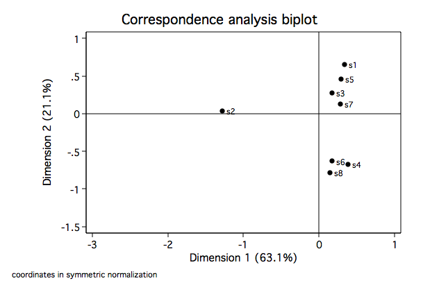
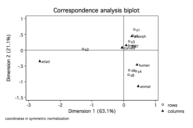
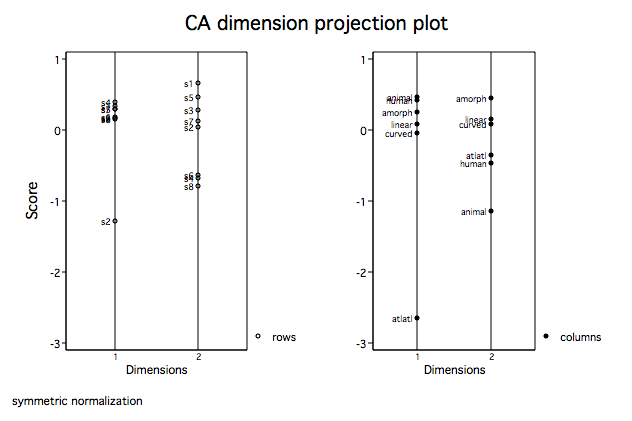 Looking at dimension 1 for columns (motifs) we see, as we suspected, that the atlatl motif
is clearly separated from the others. Further, animal and human are very close as are
linear and curved. In dimension 2 atlatl and human very close while again so are linear
and curved. For the rows we see that site 2 is clearly separated from the others on dimension
1. Let's move on to some biplots.
Looking at dimension 1 for columns (motifs) we see, as we suspected, that the atlatl motif
is clearly separated from the others. Further, animal and human are very close as are
linear and curved. In dimension 2 atlatl and human very close while again so are linear
and curved. For the rows we see that site 2 is clearly separated from the others on dimension
1. Let's move on to some biplots.
cabiplot , norow origin


cabiplot , nocol origin


cabiplot, origin rowopts(msym(Oh))
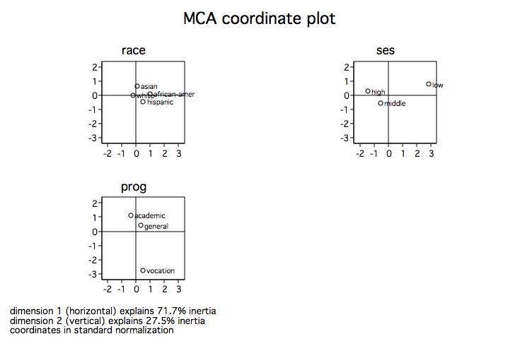
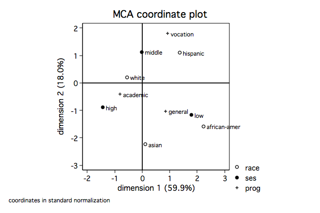
Multiple Correspondence Analysis Example
Using the mca command we will demonstrate an example of multiple correspondence analysis.
use http://www.philender.com/courses/data/hsb2, clear

mca race ses prog, dim(2)


Multiple/Joint correspondence analysis         Number of obs      =       200
                                               Total inertia      =   .066631
    Method: Burt/adjusted inertias             Number of axes     =         2

                |   principal               cumul
      Dimension |    inertia     percent   percent
    ------------+----------------------------------
          dim 1 |     .039934     59.93      59.93
          dim 2 |    .0119704     17.97      77.90
          dim 3 |    .0012654      1.90      79.80
    ------------+----------------------------------
          Total |     .066631    100.00

Statistics for column categories in standard normalization

                 |          overall          |        dimension_1
      Categories |    mass  quality   %inert |   coord   sqcorr  contrib
    -------------+---------------------------+---------------------------
    race         |                           |
        hispanic |   0.040    0.802    0.067 |   1.369    0.672    0.075
           asian |   0.018    0.621    0.027 |   0.116    0.005    0.000
    african-amer |   0.033    0.794    0.145 |   2.235    0.690    0.167
           white |   0.242    0.825    0.054 |  -0.544    0.791    0.071
    -------------+---------------------------+---------------------------
    ses          |                           |
             low |   0.078    0.770    0.220 |   1.788    0.683    0.250
          middle |   0.158    0.632    0.057 |  -0.010    0.000    0.000
            high |   0.097    0.818    0.162 |  -1.433    0.732    0.198
    -------------+---------------------------+---------------------------
    prog         |                           |
         general |   0.075    0.678    0.069 |   0.847    0.469    0.054
        academic |   0.175    0.846    0.086 |  -0.803    0.783    0.113
        vocation |   0.083    0.807    0.113 |   0.925    0.377    0.071
    ---------------------------------------------------------------------

                 |        dimension_2
      Categories |   coord   sqcorr  contrib
    -------------+---------------------------
    race         |
        hispanic |   1.099    0.130    0.048
           asian |  -2.241    0.615    0.092
    african-amer |  -1.580    0.103    0.083
           white |   0.206    0.034    0.010
    -------------+---------------------------
    ses          |
             low |  -1.173    0.088    0.108
          middle |   1.125    0.632    0.200
            high |  -0.892    0.085    0.077
    -------------+---------------------------
    prog         |
         general |  -1.033    0.209    0.080
        academic |  -0.416    0.063    0.030
        vocation |   1.803    0.430    0.271
    -----------------------------------------

mcaplot, origin


mcaplot, overlay origin
Categorical Data Analysis Course
Phil Ender 15mar08, 20dec05