
Example
use http://www.gseis.ucla.edu/courses/data/hsb2, clear
generate mathhi = math>=54
generate write2 = write^2
tabulate mathhi
mathhi | Freq. Percent Cum.
------------+-----------------------------------
0 | 108 54.00 54.00
1 | 92 46.00 100.00
------------+-----------------------------------
Total | 200 100.00
logit mathhi write, nolog
Logit estimates Number of obs = 200
LR chi2(1) = 59.60
Prob > chi2 = 0.0000
Log likelihood = -108.18989 Pseudo R2 = 0.2160
------------------------------------------------------------------------------
mathhi | Coef. Std. Err. z P>|z| [95% Conf. Interval]
-------------+----------------------------------------------------------------
write | .1422945 .0222105 6.41 0.000 .0987627 .1858262
_cons | -7.796827 1.224831 -6.37 0.000 -10.19745 -5.396203
------------------------------------------------------------------------------
predict p2
(option p assumed; Pr(mathhi))
fitstat, saving(0)
Measures of Fit for logit of mathhi
Log-Lik Intercept Only: -137.989 Log-Lik Full Model: -108.190
D(198): 216.380 LR(1): 59.598
Prob > LR: 0.000
McFadden's R2: 0.216 McFadden's Adj R2: 0.201
Maximum Likelihood R2: 0.258 Cragg & Uhler's R2: 0.344
McKelvey and Zavoina's R2: 0.356 Efron's R2: 0.286
Variance of y*: 5.109 Variance of error: 3.290
Count R2: 0.725 Adj Count R2: 0.402
AIC: 1.102 AIC*n: 220.380
BIC: -832.687 BIC': -54.299
linktest
Logit estimates Number of obs = 200
LR chi2(2) = 65.54
Prob > chi2 = 0.0000
Log likelihood = -105.21668 Pseudo R2 = 0.2375
------------------------------------------------------------------------------
mathhi | Coef. Std. Err. z P>|z| [95% Conf. Interval]
-------------+----------------------------------------------------------------
_hat | 1.270807 .2018605 6.30 0.000 .8751672 1.666446
_hatsq | .2662515 .1057033 2.52 0.012 .0590768 .4734262
_cons | -.3040576 .2107231 -1.44 0.149 -.7170672 .1089521
------------------------------------------------------------------------------
logit mathhi write write2, nolog
Logit estimates Number of obs = 200
LR chi2(2) = 65.54
Prob > chi2 = 0.0000
Log likelihood = -105.21668 Pseudo R2 = 0.2375
------------------------------------------------------------------------------
mathhi | Coef. Std. Err. z P>|z| [95% Conf. Interval]
-------------+----------------------------------------------------------------
write | -.4099542 .2153784 -1.90 0.057 -.8320882 .0121797
write2 | .005391 .0021403 2.52 0.012 .0011962 .0095858
_cons | 5.97325 5.316722 1.12 0.261 -4.447334 16.39383
------------------------------------------------------------------------------
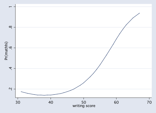
postgr3 write, asis(write write2) gen(p1)
Variables left asis: write write2
(option p assumed; Pr(mathhi))
 linktest
Logit estimates Number of obs = 200
LR chi2(2) = 65.70
Prob > chi2 = 0.0000
Log likelihood = -105.14092 Pseudo R2 = 0.2380
------------------------------------------------------------------------------
mathhi | Coef. Std. Err. z P>|z| [95% Conf. Interval]
-------------+----------------------------------------------------------------
_hat | 1.001082 .1450353 6.90 0.000 .7168177 1.285345
_hatsq | -.0459454 .116897 -0.39 0.694 -.2750592 .1831685
_cons | .0639112 .2373879 0.27 0.788 -.4013605 .529183
------------------------------------------------------------------------------
fitstat, using(0)
Measures of Fit for logit of mathhi
Current Saved Difference
Model: logit logit
N: 200 200 0
Log-Lik Intercept Only: -137.989 -137.989 0.000
Log-Lik Full Model: -105.217 -108.190 2.973
D: 210.433(197) 216.380(198) 5.946(1)
LR: 65.544(2) 59.598(1) 5.946(1)
Prob > LR: 0.000 0.000 0.015
McFadden's R2: 0.237 0.216 0.022
McFadden's Adj R2: 0.216 0.201 0.014
Maximum Likelihood R2: 0.279 0.258 0.022
Cragg & Uhler's R2: 0.373 0.344 0.029
McKelvey and Zavoina's R2: 0.362 0.356 0.006
Efron's R2: 0.297 0.286 0.011
Variance of y*: 5.155 5.109 0.046
Variance of error: 3.290 3.290 0.000
Count R2: 0.740 0.725 0.015
Adj Count R2: 0.435 0.402 0.033
AIC: 1.082 1.102 -0.020
AIC*n: 216.433 220.380 -3.946
BIC: -833.335 -832.687 -0.648
BIC': -54.948 -54.299 -0.648
Difference of 0.648 in BIC' provides weak support for current model.
Note: p-value for difference in LR is only valid if models are nested.
Difference of 0.648 in BIC' provides weak support for saved model.
Note: p-value for difference in LR is only valid if models are nested.
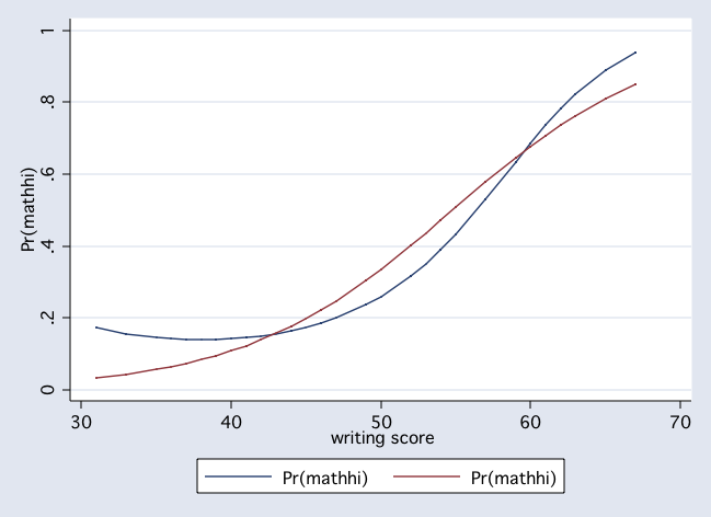
scatter p1 p2 write, con(l l) msym(i i) sort
linktest
Logit estimates Number of obs = 200
LR chi2(2) = 65.70
Prob > chi2 = 0.0000
Log likelihood = -105.14092 Pseudo R2 = 0.2380
------------------------------------------------------------------------------
mathhi | Coef. Std. Err. z P>|z| [95% Conf. Interval]
-------------+----------------------------------------------------------------
_hat | 1.001082 .1450353 6.90 0.000 .7168177 1.285345
_hatsq | -.0459454 .116897 -0.39 0.694 -.2750592 .1831685
_cons | .0639112 .2373879 0.27 0.788 -.4013605 .529183
------------------------------------------------------------------------------
fitstat, using(0)
Measures of Fit for logit of mathhi
Current Saved Difference
Model: logit logit
N: 200 200 0
Log-Lik Intercept Only: -137.989 -137.989 0.000
Log-Lik Full Model: -105.217 -108.190 2.973
D: 210.433(197) 216.380(198) 5.946(1)
LR: 65.544(2) 59.598(1) 5.946(1)
Prob > LR: 0.000 0.000 0.015
McFadden's R2: 0.237 0.216 0.022
McFadden's Adj R2: 0.216 0.201 0.014
Maximum Likelihood R2: 0.279 0.258 0.022
Cragg & Uhler's R2: 0.373 0.344 0.029
McKelvey and Zavoina's R2: 0.362 0.356 0.006
Efron's R2: 0.297 0.286 0.011
Variance of y*: 5.155 5.109 0.046
Variance of error: 3.290 3.290 0.000
Count R2: 0.740 0.725 0.015
Adj Count R2: 0.435 0.402 0.033
AIC: 1.082 1.102 -0.020
AIC*n: 216.433 220.380 -3.946
BIC: -833.335 -832.687 -0.648
BIC': -54.948 -54.299 -0.648
Difference of 0.648 in BIC' provides weak support for current model.
Note: p-value for difference in LR is only valid if models are nested.
Difference of 0.648 in BIC' provides weak support for saved model.
Note: p-value for difference in LR is only valid if models are nested.
scatter p1 p2 write, con(l l) msym(i i) sort
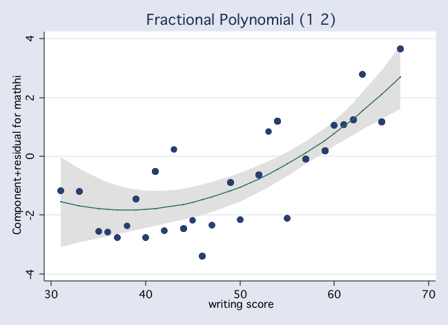
Next, we will use the fracpoly command to do the polynomial logistic regression.
fracpoly logit mathhi write 1 2, nolog
-> gen double Iwrit__1 = X-5.277 if e(sample)
-> gen double Iwrit__2 = X^2-27.85 if e(sample)
   (where: X = write/10)

Logit estimates                                   Number of obs   =        200
                                                  LR chi2(2)      =      65.54
                                                  Prob > chi2     =     0.0000
Log likelihood = -105.21668                       Pseudo R2       =     0.2375

------------------------------------------------------------------------------
      mathhi |      Coef.   Std. Err.      z    P>|z|     [95% Conf. Interval]
-------------+----------------------------------------------------------------
    Iwrit__1 |  -4.099542   2.153784    -1.90   0.057    -8.320882    .1217973
    Iwrit__2 |   .5390984   .2140251     2.52   0.012     .1196169    .9585798
       _cons |  -.6471137   .2288751    -2.83   0.005    -1.095701   -.1985267
------------------------------------------------------------------------------
Deviance:  210.433.

fracplot write
Finally, we will use fracpoly again but this time let it search for the best
fitting polynomial. In this case, it used write and write-2
fracpoly logit mathhi write
........
-> gen double Iwrit__1 = X^-2-.0359 if e(sample)
-> gen double Iwrit__2 = X-5.277 if e(sample)
   (where: X = write/10)

Logit estimates                                   Number of obs   =        200
                                                  LR chi2(2)      =      66.01
                                                  Prob > chi2     =     0.0000
Log likelihood = -104.98407                       Pseudo R2       =     0.2392

------------------------------------------------------------------------------
      mathhi |      Coef.   Std. Err.      z    P>|z|     [95% Conf. Interval]
-------------+----------------------------------------------------------------
    Iwrit__1 |   86.12373   31.13893     2.77   0.006     25.09256    147.1549
    Iwrit__2 |   2.915556   .6256198     4.66   0.000     1.689364    4.141748
       _cons |  -.5831283   .2112336    -2.76   0.006    -.9971387    -.169118
------------------------------------------------------------------------------
Deviance: 209.9681. Best powers of write among 44 models fit: -2 1.

linktest


Logit estimates                                   Number of obs   =        200
                                                  LR chi2(2)      =      66.02
                                                  Prob > chi2     =     0.0000
Log likelihood = -104.98113                       Pseudo R2       =     0.2392

------------------------------------------------------------------------------
      mathhi |      Coef.   Std. Err.      z    P>|z|     [95% Conf. Interval]
-------------+----------------------------------------------------------------
        _hat |   1.001922   .1473193     6.80   0.000     .7131815    1.290663
      _hatsq |   .0093415   .1219907     0.08   0.939    -.2297559    .2484389
       _cons |  -.0127298    .238401    -0.05   0.957    -.4799871    .4545275
------------------------------------------------------------------------------


fitstat

Measures of Fit for logit of mathhi

Log-Lik Intercept Only:     -137.989     Log-Lik Full Model:         -104.984
D(197):                      209.968     LR(2):                        66.009
                                         Prob > LR:                     0.000
McFadden's R2:                 0.239     McFadden's Adj R2:             0.217
Maximum Likelihood R2:         0.281     Cragg & Uhler's R2:            0.376
McKelvey and Zavoina's R2:     0.360     Efron's R2:                    0.300
Variance of y*:                5.141     Variance of error:             3.290
Count R2:                      0.740     Adj Count R2:                  0.435
AIC:                           1.080     AIC*n:                       215.968
BIC:                        -833.800     BIC':                        -55.413
Categorical Data Analysis Course
Phil Ender