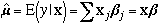
In OLS regression, we use linear combinations of predictor (independent) variables to compute expected values of the response (dependent) variable.
The matrix formulation for OLS regression looks like this
Stata Program using Matrix Arithmetic
program define matreg2, eclass
  version 6.0

    syntax varlist(min=2 numeric) [if] [in] [, Level(integer $S_level)]
    marksample touse                       /* mark cases in the sample */
    tokenize "`varlist'"

    quietly matrix accum sscp = `varlist' if `touse'
    local nobs = r(N)
    local df = `nobs' - (rowsof(sscp) - 1) /* df residual */

    matrix XX = sscp[2...,2...]            /* X'X */
    matrix Xy = sscp[1,2...]               /* X'y */

    matrix b = Xy * syminv(XX)             /* (X'X)-1X'y */
    local k = colsof(b)                    /* number of coefs */
    matrix hat = Xy * b'
    matrix V = syminv(XX) * (sscp[1,1] - hat[1,1])/`df'

    estimates post b V, dof(`df') obs(`nobs') depname(`1') /*
      */ esample(`touse')
    est local depvar "`1'"
    est local cmd "matreg"

    display
    estimates display, level(`level')

  matrix drop sscp XX Xy hat
end
Example using matreg2
use http://www.ats.ucla.edu/stat/data/hsbdemo, clear

regress write read female

matreg2 write read female
Assumptions in OLS Regression
Linearity - The expected value of y is linearly related to the x's through the β parameters. Specification errors result when there is a nonlinear relationship.
Independence - The independence of the x's and ε is necessary in order to identify the unknown β parameters, that is, in order to be able to solve for the β's
ε are i.i.d. - The assumption is that the ε's are independent and identically distributed which implies there should be no heterogeneity of variance and no autocorrelation among the residuals.
All relevant variables are in the model - A specification error can occur when the model does not contain all of the relevant variables. As a corollary, a specification error can occur when irrelevant variables are included in the model.
x's are measured without error - The independent variables are measured without error.
Normality* - If we wish to draw statistical inferences we need to add the further assumption that the ε are normally distributed.
Example
use http://www.ats.ucla.edu/stat/data/hsbdemo, clear
describe
Contains data from http://www.gseis.ucla.edu/courses/data/hsb2.dta
obs: 200 highschool and beyond (200
cases)
vars: 11 21 Jun 2000 08:54
size: 9,600 (99.8% of memory free)
-------------------------------------------------------------------------------
1. id float %9.0g
2. female float %9.0g fl
3. race float %12.0g rl
4. ses float %9.0g sl
5. schtyp float %9.0g scl type of school
6. prog float %9.0g sel type of program
7. read float %9.0g reading score
8. write float %9.0g writing score
9. math float %9.0g math score
10. science float %9.0g science score
11. socst float %9.0g social studies score
-------------------------------------------------------------------------------
summarize
Variable | Obs Mean Std. Dev. Min Max
---------+-----------------------------------------------------
id | 200 100.5 57.87918 1 200
female | 200 .545 .4992205 0 1
race | 200 3.43 1.039472 1 4
ses | 200 2.055 .7242914 1 3
schtyp | 200 1.16 .367526 1 2
prog | 200 2.025 .6904772 1 3
read | 200 52.23 10.25294 28 76
write | 200 52.775 9.478586 31 67
math | 200 52.645 9.368448 33 75
science | 200 51.85 9.900891 26 74
socst | 200 52.405 10.73579 26 71
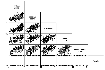
corr write read math science socst female
(obs=200)
| write read math science socst female
-------------+------------------------------------------------------
write | 1.0000
read | 0.5968 1.0000
math | 0.6174 0.6623 1.0000
science | 0.5704 0.6302 0.6307 1.0000
socst | 0.6048 0.6215 0.5445 0.4651 1.0000
female | 0.2565 -0.0531 -0.0293 -0.1277 0.0524 1.0000
pcorr write read math science socst female
(obs=200)
Partial correlation of write with
Variable | Corr. Sig.
-------------+------------------
read | 0.1373 0.055
math | 0.2468 0.000
science | 0.2751 0.000
socst | 0.2974 0.000
female | 0.4107 0.000
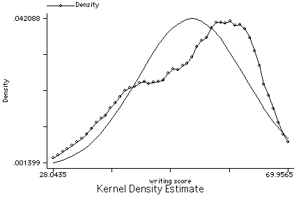
kdensity write, normal
 graph read math science socst female write, matrix half
 tab1 female prog
-> tabulation of female
female | Freq. Percent Cum.
------------+-----------------------------------
male | 91 45.50 45.50
female | 109 54.50 100.00
------------+-----------------------------------
Total | 200 100.00
-> tabulation of prog
type of |
program | Freq. Percent Cum.
------------+-----------------------------------
general | 45 22.50 22.50
academic | 105 52.50 75.00
vocation | 50 25.00 100.00
------------+-----------------------------------
Total | 200 100.00
regress write read math female i.prog
Source | SS df MS Number of obs = 200
-------------+------------------------------ F( 5, 194) = 45.01
Model | 9602.28627 5 1920.45725 Prob > F = 0.0000
Residual | 8276.58873 194 42.6628285 R-squared = 0.5371
-------------+------------------------------ Adj R-squared = 0.5251
Total | 17878.875 199 89.843593 Root MSE = 6.5317
------------------------------------------------------------------------------
write | Coef. Std. Err. t P>|t| [95% Conf. Interval]
-------------+----------------------------------------------------------------
read | .3069424 .0611262 5.02 0.000 .1863852 .4274996
math | .3603705 .0690064 5.22 0.000 .2242715 .4964695
female | 5.384982 .929572 5.79 0.000 3.551617 7.218346
|
prog |
2 | .436372 1.230379 0.35 0.723 -1.990265 2.863009
3 | -2.219748 1.359353 -1.63 0.104 -4.900756 .4612603
|
_cons | 15.16272 3.225088 4.70 0.000 8.801985 21.52346
------------------------------------------------------------------------------
test 2.prog 3.prog
( 1) Iprog_2 = 0.0
( 2) Iprog_3 = 0.0
F( 2, 194) = 2.31
Prob > F = 0.1022
regress write read math female
Source | SS df MS Number of obs = 200
---------+------------------------------ F( 3, 196) = 72.52
Model | 9405.34864 3 3135.11621 Prob > F = 0.0000
Residual | 8473.52636 196 43.2322773 R-squared = 0.5261
---------+------------------------------ Adj R-squared = 0.5188
Total | 17878.875 199 89.843593 Root MSE = 6.5751
------------------------------------------------------------------------------
write | Coef. Std. Err. t P>|t| [95% Conf. Interval]
---------+--------------------------------------------------------------------
read | .3252389 .0607348 5.355 0.000 .2054613 .4450166
math | .3974826 .0664037 5.986 0.000 .266525 .5284401
female | 5.44337 .9349987 5.822 0.000 3.59942 7.287319
_cons | 11.89566 2.862845 4.155 0.000 6.249728 17.5416
------------------------------------------------------------------------------
listcoef /* from Long & Freese - findit spostado */
regress (N=200): Unstandardized and Standardized Estimates
Observed SD: 9.478586
SD of Error: 6.5751257
---------------------------------------------------------------------------
write | b t P>|t| bStdX bStdY bStdXY SDofX
---------+-----------------------------------------------------------------
read | 0.32524 5.355 0.000 3.3347 0.0343 0.3518 10.2529
math | 0.39748 5.986 0.000 3.7238 0.0419 0.3929 9.3684
female | 5.44337 5.822 0.000 2.7174 0.5743 0.2867 0.4992
---------------------------------------------------------------------------
linktest
Source | SS df MS Number of obs = 200
---------+------------------------------ F( 2, 197) = 116.16
Model | 9674.70222 2 4837.35111 Prob > F = 0.0000
Residual | 8204.17278 197 41.6455471 R-squared = 0.5411
---------+------------------------------ Adj R-squared = 0.5365
Total | 17878.875 199 89.843593 Root MSE = 6.4533
------------------------------------------------------------------------------
write | Coef. Std. Err. t P>|t| [95% Conf. Interval]
---------+--------------------------------------------------------------------
_hat | 3.306865 .9095168 3.636 0.000 1.513226 5.100504
_hatsq | -.0215942 .008491 -2.543 0.012 -.0383392 -.0048492
_cons | -60.58511 24.08436 -2.516 0.013 -108.0814 -13.08885
------------------------------------------------------------------------------
ovtest
Ramsey RESET test using powers of the fitted values of write
Ho: model has no omitted variables
F(3, 193) = 3.06
Prob > F = 0.0295
whitetst /* downloaded via the Internet - findit whitetst */
White's general test statistic : 15.17126 Chi-sq( 8) P-value = .0559
regress write read math female science socst
Source | SS df MS Number of obs = 200
---------+------------------------------ F( 5, 194) = 58.60
Model | 10756.9244 5 2151.38488 Prob > F = 0.0000
Residual | 7121.9506 194 36.7110855 R-squared = 0.6017
---------+------------------------------ Adj R-squared = 0.5914
Total | 17878.875 199 89.843593 Root MSE = 6.059
------------------------------------------------------------------------------
write | Coef. Std. Err. t P>|t| [95% Conf. Interval]
---------+--------------------------------------------------------------------
read | .1254123 .0649598 1.931 0.055 -.0027059 .2535304
math | .2380748 .0671266 3.547 0.000 .1056832 .3704665
female | 5.492502 .8754227 6.274 0.000 3.765935 7.21907
science | .2419382 .0606997 3.986 0.000 .1222221 .3616542
socst | .2292644 .0528361 4.339 0.000 .1250575 .3334713
_cons | 6.138759 2.808423 2.186 0.030 .599798 11.67772
------------------------------------------------------------------------------
linktest
Source | SS df MS Number of obs = 200
---------+------------------------------ F( 2, 197) = 155.20
Model | 10937.2369 2 5468.61843 Prob > F = 0.0000
Residual | 6941.63813 197 35.2367418 R-squared = 0.6117
---------+------------------------------ Adj R-squared = 0.6078
Total | 17878.875 199 89.843593 Root MSE = 5.9361
------------------------------------------------------------------------------
write | Coef. Std. Err. t P>|t| [95% Conf. Interval]
---------+--------------------------------------------------------------------
_hat | 2.577803 .6998344 3.683 0.000 1.197674 3.957931
_hatsq | -.0150213 .0066404 -2.262 0.025 -.0281166 -.0019259
_cons | -40.62334 18.21521 -2.230 0.027 -76.54518 -4.701504
------------------------------------------------------------------------------
ovtest
Ramsey RESET test using powers of the fitted values of write
Ho: model has no omitted variables
F(3, 191) = 2.03
Prob > F = 0.1117
whitetst /* downloaded via the Internet - findit whitetst */
White's general test statistic : 23.69338 Chi-sq(19) P-value = .2082
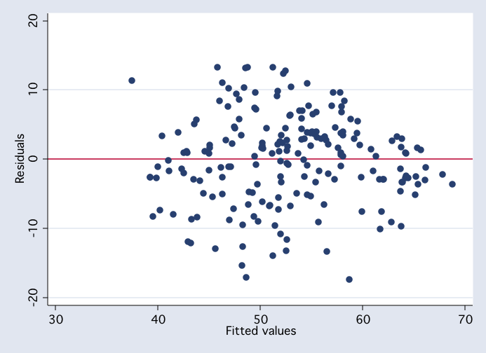
rvfplot, yline(0) jitter(2)
tab1 female prog
-> tabulation of female
female | Freq. Percent Cum.
------------+-----------------------------------
male | 91 45.50 45.50
female | 109 54.50 100.00
------------+-----------------------------------
Total | 200 100.00
-> tabulation of prog
type of |
program | Freq. Percent Cum.
------------+-----------------------------------
general | 45 22.50 22.50
academic | 105 52.50 75.00
vocation | 50 25.00 100.00
------------+-----------------------------------
Total | 200 100.00
regress write read math female i.prog
Source | SS df MS Number of obs = 200
-------------+------------------------------ F( 5, 194) = 45.01
Model | 9602.28627 5 1920.45725 Prob > F = 0.0000
Residual | 8276.58873 194 42.6628285 R-squared = 0.5371
-------------+------------------------------ Adj R-squared = 0.5251
Total | 17878.875 199 89.843593 Root MSE = 6.5317
------------------------------------------------------------------------------
write | Coef. Std. Err. t P>|t| [95% Conf. Interval]
-------------+----------------------------------------------------------------
read | .3069424 .0611262 5.02 0.000 .1863852 .4274996
math | .3603705 .0690064 5.22 0.000 .2242715 .4964695
female | 5.384982 .929572 5.79 0.000 3.551617 7.218346
|
prog |
2 | .436372 1.230379 0.35 0.723 -1.990265 2.863009
3 | -2.219748 1.359353 -1.63 0.104 -4.900756 .4612603
|
_cons | 15.16272 3.225088 4.70 0.000 8.801985 21.52346
------------------------------------------------------------------------------
test 2.prog 3.prog
( 1) Iprog_2 = 0.0
( 2) Iprog_3 = 0.0
F( 2, 194) = 2.31
Prob > F = 0.1022
regress write read math female
Source | SS df MS Number of obs = 200
---------+------------------------------ F( 3, 196) = 72.52
Model | 9405.34864 3 3135.11621 Prob > F = 0.0000
Residual | 8473.52636 196 43.2322773 R-squared = 0.5261
---------+------------------------------ Adj R-squared = 0.5188
Total | 17878.875 199 89.843593 Root MSE = 6.5751
------------------------------------------------------------------------------
write | Coef. Std. Err. t P>|t| [95% Conf. Interval]
---------+--------------------------------------------------------------------
read | .3252389 .0607348 5.355 0.000 .2054613 .4450166
math | .3974826 .0664037 5.986 0.000 .266525 .5284401
female | 5.44337 .9349987 5.822 0.000 3.59942 7.287319
_cons | 11.89566 2.862845 4.155 0.000 6.249728 17.5416
------------------------------------------------------------------------------
listcoef /* from Long & Freese - findit spostado */
regress (N=200): Unstandardized and Standardized Estimates
Observed SD: 9.478586
SD of Error: 6.5751257
---------------------------------------------------------------------------
write | b t P>|t| bStdX bStdY bStdXY SDofX
---------+-----------------------------------------------------------------
read | 0.32524 5.355 0.000 3.3347 0.0343 0.3518 10.2529
math | 0.39748 5.986 0.000 3.7238 0.0419 0.3929 9.3684
female | 5.44337 5.822 0.000 2.7174 0.5743 0.2867 0.4992
---------------------------------------------------------------------------
linktest
Source | SS df MS Number of obs = 200
---------+------------------------------ F( 2, 197) = 116.16
Model | 9674.70222 2 4837.35111 Prob > F = 0.0000
Residual | 8204.17278 197 41.6455471 R-squared = 0.5411
---------+------------------------------ Adj R-squared = 0.5365
Total | 17878.875 199 89.843593 Root MSE = 6.4533
------------------------------------------------------------------------------
write | Coef. Std. Err. t P>|t| [95% Conf. Interval]
---------+--------------------------------------------------------------------
_hat | 3.306865 .9095168 3.636 0.000 1.513226 5.100504
_hatsq | -.0215942 .008491 -2.543 0.012 -.0383392 -.0048492
_cons | -60.58511 24.08436 -2.516 0.013 -108.0814 -13.08885
------------------------------------------------------------------------------
ovtest
Ramsey RESET test using powers of the fitted values of write
Ho: model has no omitted variables
F(3, 193) = 3.06
Prob > F = 0.0295
whitetst /* downloaded via the Internet - findit whitetst */
White's general test statistic : 15.17126 Chi-sq( 8) P-value = .0559
regress write read math female science socst
Source | SS df MS Number of obs = 200
---------+------------------------------ F( 5, 194) = 58.60
Model | 10756.9244 5 2151.38488 Prob > F = 0.0000
Residual | 7121.9506 194 36.7110855 R-squared = 0.6017
---------+------------------------------ Adj R-squared = 0.5914
Total | 17878.875 199 89.843593 Root MSE = 6.059
------------------------------------------------------------------------------
write | Coef. Std. Err. t P>|t| [95% Conf. Interval]
---------+--------------------------------------------------------------------
read | .1254123 .0649598 1.931 0.055 -.0027059 .2535304
math | .2380748 .0671266 3.547 0.000 .1056832 .3704665
female | 5.492502 .8754227 6.274 0.000 3.765935 7.21907
science | .2419382 .0606997 3.986 0.000 .1222221 .3616542
socst | .2292644 .0528361 4.339 0.000 .1250575 .3334713
_cons | 6.138759 2.808423 2.186 0.030 .599798 11.67772
------------------------------------------------------------------------------
linktest
Source | SS df MS Number of obs = 200
---------+------------------------------ F( 2, 197) = 155.20
Model | 10937.2369 2 5468.61843 Prob > F = 0.0000
Residual | 6941.63813 197 35.2367418 R-squared = 0.6117
---------+------------------------------ Adj R-squared = 0.6078
Total | 17878.875 199 89.843593 Root MSE = 5.9361
------------------------------------------------------------------------------
write | Coef. Std. Err. t P>|t| [95% Conf. Interval]
---------+--------------------------------------------------------------------
_hat | 2.577803 .6998344 3.683 0.000 1.197674 3.957931
_hatsq | -.0150213 .0066404 -2.262 0.025 -.0281166 -.0019259
_cons | -40.62334 18.21521 -2.230 0.027 -76.54518 -4.701504
------------------------------------------------------------------------------
ovtest
Ramsey RESET test using powers of the fitted values of write
Ho: model has no omitted variables
F(3, 191) = 2.03
Prob > F = 0.1117
whitetst /* downloaded via the Internet - findit whitetst */
White's general test statistic : 23.69338 Chi-sq(19) P-value = .2082
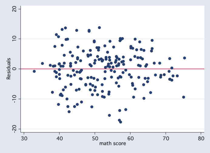
rvfplot, yline(0) jitter(2)
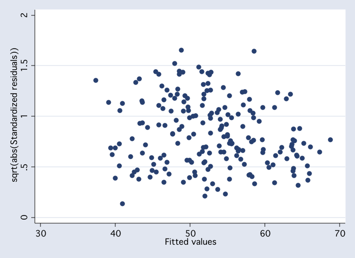
 rvfplot2, rsta rscale(sqrt(abs(X))) jitter(2) /* downloaded via the Internet - findit rvfplot2 */
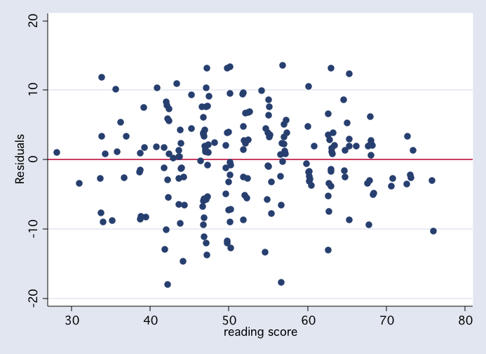
 rvpplot read, yline(0) jitter(2)
 rvpplot math, yline(0) jitter(2)
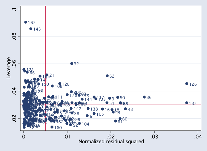
 lvr2plot, mlabel(id)
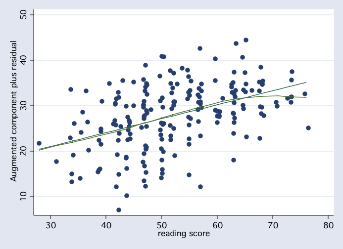
 acprplot read, lowess jitter(2)
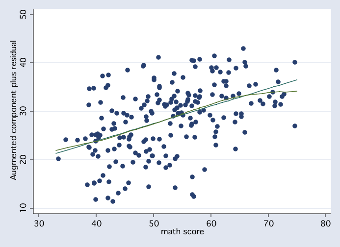
 acprplot math, lowess jitter(2)
 predict e, resid
predict rstu, rstu
predict h, hat
predict d, cooksd
dfbeta
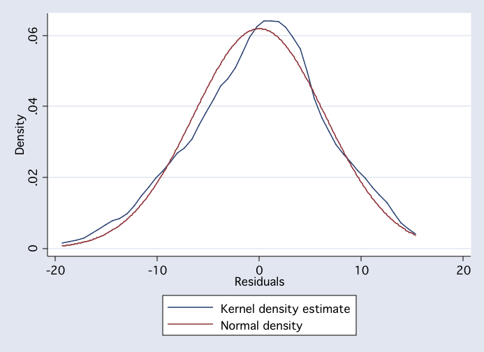
kdensity e, normal
predict e, resid
predict rstu, rstu
predict h, hat
predict d, cooksd
dfbeta
kdensity e, normal
 list id rstu h d if abs(rstu)>2
id rstu h d
6. 126 -2.911042 .0306996 .0430727
21. 86 -2.159355 .0471286 .0377245
42. 187 -2.801592 .012483 .0159722
71. 52 -2.102624 .0243733 .0180889
119. 38 2.225437 .0551778 .0472426
127. 104 2.12688 .0164202 .0123619
137. 30 2.077298 .0271825 .0197581
156. 44 2.543062 .0270288 .0291219
160. 83 2.393317 .0556316 .0549
list id rstu h d if h>(2*5+2)/200
id rstu h d
38. 167 .2202322 .1129052 .0010339
74. 198 1.536736 .0626366 .0261174
140. 170 .615899 .0624444 .0042243
174. 165 .4212941 .0611342 .0019344
190. 150 -1.481232 .096819 .0389597
list id rstu h d if d>4/200
id rstu h d
6. 126 -2.911042 .0306996 .0430727
21. 86 -2.159355 .0471286 .0377245
48. 24 1.995236 .0473758 .0324974
57. 3 1.937731 .0350953 .0224428
74. 198 1.536736 .0626366 .0261174
119. 38 2.225437 .0551778 .0472426
144. 81 -1.843365 .0358387 .020794
156. 44 2.543062 .0270288 .0291219
160. 83 2.393317 .0556316 .0549
190. 150 -1.481232 .096819 .0389597
196. 89 -1.771696 .0422013 .022799
global a = 2/sqrt(200)
list id DFread DFmath DFfemale DFscienc DFsocst if abs(DFread)>$a | abs(DFmat
> h)>$a | abs(DFfemale)>$a | abs(DFscienc)>$a | abs(DFsocst)>$a
id DFread DFmath DFfemale DFscienc DFsocst
3. 51 -.0515056 -.014398 -.0626913 .1468613 .0604603
6. 126 .3206731 -.3131511 .2656341 .1226514 -.0953587
9. 175 -.1430553 -.0606901 .1151235 .1475843 -.0274637
21. 86 .0980499 -.1335611 .1154265 -.1851264 .3323804
24. 62 .1088972 -.2401099 -.1083746 .1068583 .1222108
33. 50 -.0349264 -.2120363 -.1395483 .0761597 .1938863
42. 187 -.0829706 -.0537039 -.1999146 -.0223069 .1177308
48. 24 -.0347862 .3662628 -.1715901 -.2201185 -.1457788
55. 60 -.0166963 -.1514111 -.1222548 .1529634 .1088403
57. 3 .1622479 -.2598199 -.1198602 .1595348 .0001202
71. 52 .1520838 .0367512 -.1116373 -.0425734 -.2523727
74. 198 -.0183564 -.0090244 .1612648 .2468743 -.2791837
76. 186 .0420188 .0984112 .0757014 -.0094653 -.1424532
81. 103 -.2083498 .0167522 .0938213 .0255195 .0635244
102. 189 -.1159227 .2095263 -.1127493 -.0281062 -.0706801
109. 41 .0333516 .1437377 .1196449 -.0881504 -.1007374
110. 185 .1353671 -.012621 -.0607331 .0121166 -.1576565
113. 46 .081996 .0152051 .0863532 -.173799 -.0803784
119. 38 -.0400404 .1510486 -.2598652 -.4282386 .2007007
127. 104 .0250837 .0949613 -.147284 .0018263 -.1392599
134. 159 .0034894 .0056749 -.1422074 -.0914222 .1120808
137. 30 -.0398192 -.033048 .0875061 -.1889646 .1237977
139. 200 .0064968 -.2036626 .1237578 .0268331 -.0128401
144. 81 -.1431379 -.0059714 .0933692 -.1201475 .2423838
154. 133 -.1600672 .0340288 .0858443 .1343556 .1441613
155. 98 .1430875 -.0204046 .1143515 .0250712 -.2119574
156. 44 .1320848 .0129432 .1237565 -.3070052 -.0404682
160. 83 .2011815 -.2430923 .2346933 .2569073 -.3997001
162. 18 -.1112641 -.0427497 .1235689 .1017029 .191583
166. 117 -.143197 -.0619351 -.10833 .0033026 .1643665
169. 153 .0994511 .0801062 .1757641 .0828039 -.1559673
186. 16 -.110932 -.0121689 .1209114 .1604108 .1236713
190. 150 .1878171 -.0798048 .0538377 -.3412711 .2439169
192. 142 .0095487 -.086411 -.0723012 .1508893 -.0155141
196. 89 .1260335 .0847179 -.1482973 -.2127656 .1433555
diag, id(id) /* downloaded via the Internet - findit diag */
Summary statistics for Leverage/Residuals (Panel 1) and dfbetas (Panel 2)
Signals lists the obs that warrant attention (criteria: see online help)
Variable | Obs Mean Std. Dev. Min Max %Signals
---------+--------------------------------------------------------------------
_hat | 200 .03 .0137395 .0105296 .1129052 0.0250
_rstu | 200 5.13e-06 1.00769 -2.911042 2.543062 0.0800
_dfits | 200 .0013422 .1790669 -.5180668 .5808853 0.0350
_cooksd | 200 .0052647 .0085635 9.85e-08 .0549 0.0550
_welsch | 200 .0194215 2.574987 -7.423061 8.432303 0.0100
_covrati | 200 1.031876 .0446067 .8223104 1.161025 0.0250
---------+--------------------------------------------------------------------
read | 200 .0001225 .0663172 -.2083498 .3206731 0.0550
math | 200 -.0001245 .0732815 -.3131511 .3662628 0.0550
female | 200 .0000807 .0748938 -.2598652 .2656341 0.0500
science | 200 -.000107 .0791052 -.4282386 .2569073 0.0800
socst | 200 .0000599 .0793047 -.3997001 .3323804 0.0850
---------+--------------------------------------------------------------------
Frequency distribution of #signals
_Signals | Freq. Percent Cum.
------------+-----------------------------------
0 | 159 79.50 79.50
1 | 17 8.50 88.00
2 | 9 4.50 92.50
3 | 4 2.00 94.50
4 | 3 1.50 96.00
5 | 2 1.00 97.00
6 | 3 1.50 98.50
7 | 1 0.50 99.00
8 | 1 0.50 99.50
9 | 1 0.50 100.00
------------+-----------------------------------
Total | 200 100.00
Observations with #signals >= 1
-------------------------------------------------------------------------------
_Signals #signals for the observation
_diag signals for _HAT _RSTU _DFITS _COOKSD _WELSCH _COVRATIO
_dfbeta signals for dbetas of read math female _Iprog_2 _Iprog_3
+-----------------------------------+
| id _Signals _diag _dfbeta |
|-----------------------------------|
| 111 1 000000 00001 |
| 8 1 000000 10000 |
| 200 1 000000 01000 |
| 128 1 000000 00010 |
| 121 1 000001 00000 |
|-----------------------------------|
| 142 1 000000 00001 |
| 108 1 000000 00001 |
| 138 1 000000 00001 |
| 30 1 000000 00010 |
| 103 1 000000 10000 |
|-----------------------------------|
| 63 1 000000 00010 |
| 170 2 000000 11000 |
| 92 2 000000 00011 |
| 105 2 000000 01010 |
| 81 2 010000 00100 |
|-----------------------------------|
| 109 2 000000 00011 |
| 143 2 100001 00000 |
| 175 2 000000 00011 |
| 167 2 100001 00000 |
| 60 2 010000 00100 |
|-----------------------------------|
| 44 2 010000 00001 |
| 178 2 000000 01001 |
| 144 2 000000 00011 |
| 21 2 000000 01010 |
| 133 3 010000 01001 |
|-----------------------------------|
| 18 3 010000 00101 |
| 16 3 010000 00101 |
| 43 4 010100 01010 |
| 51 4 010100 00011 |
| 32 5 101100 01001 |
|-----------------------------------|
| 85 5 010100 00111 |
| 117 5 011100 00101 |
| 187 6 010101 00111 |
| 3 6 011100 11100 |
| 62 7 011100 11011 |
|-----------------------------------|
| 50 7 011100 01111 |
| 83 7 011100 11101 |
| 126 8 010101 11111 |
| 86 8 010101 11111 |
+-----------------------------------+
list id rstu h d if abs(rstu)>2
id rstu h d
6. 126 -2.911042 .0306996 .0430727
21. 86 -2.159355 .0471286 .0377245
42. 187 -2.801592 .012483 .0159722
71. 52 -2.102624 .0243733 .0180889
119. 38 2.225437 .0551778 .0472426
127. 104 2.12688 .0164202 .0123619
137. 30 2.077298 .0271825 .0197581
156. 44 2.543062 .0270288 .0291219
160. 83 2.393317 .0556316 .0549
list id rstu h d if h>(2*5+2)/200
id rstu h d
38. 167 .2202322 .1129052 .0010339
74. 198 1.536736 .0626366 .0261174
140. 170 .615899 .0624444 .0042243
174. 165 .4212941 .0611342 .0019344
190. 150 -1.481232 .096819 .0389597
list id rstu h d if d>4/200
id rstu h d
6. 126 -2.911042 .0306996 .0430727
21. 86 -2.159355 .0471286 .0377245
48. 24 1.995236 .0473758 .0324974
57. 3 1.937731 .0350953 .0224428
74. 198 1.536736 .0626366 .0261174
119. 38 2.225437 .0551778 .0472426
144. 81 -1.843365 .0358387 .020794
156. 44 2.543062 .0270288 .0291219
160. 83 2.393317 .0556316 .0549
190. 150 -1.481232 .096819 .0389597
196. 89 -1.771696 .0422013 .022799
global a = 2/sqrt(200)
list id DFread DFmath DFfemale DFscienc DFsocst if abs(DFread)>$a | abs(DFmat
> h)>$a | abs(DFfemale)>$a | abs(DFscienc)>$a | abs(DFsocst)>$a
id DFread DFmath DFfemale DFscienc DFsocst
3. 51 -.0515056 -.014398 -.0626913 .1468613 .0604603
6. 126 .3206731 -.3131511 .2656341 .1226514 -.0953587
9. 175 -.1430553 -.0606901 .1151235 .1475843 -.0274637
21. 86 .0980499 -.1335611 .1154265 -.1851264 .3323804
24. 62 .1088972 -.2401099 -.1083746 .1068583 .1222108
33. 50 -.0349264 -.2120363 -.1395483 .0761597 .1938863
42. 187 -.0829706 -.0537039 -.1999146 -.0223069 .1177308
48. 24 -.0347862 .3662628 -.1715901 -.2201185 -.1457788
55. 60 -.0166963 -.1514111 -.1222548 .1529634 .1088403
57. 3 .1622479 -.2598199 -.1198602 .1595348 .0001202
71. 52 .1520838 .0367512 -.1116373 -.0425734 -.2523727
74. 198 -.0183564 -.0090244 .1612648 .2468743 -.2791837
76. 186 .0420188 .0984112 .0757014 -.0094653 -.1424532
81. 103 -.2083498 .0167522 .0938213 .0255195 .0635244
102. 189 -.1159227 .2095263 -.1127493 -.0281062 -.0706801
109. 41 .0333516 .1437377 .1196449 -.0881504 -.1007374
110. 185 .1353671 -.012621 -.0607331 .0121166 -.1576565
113. 46 .081996 .0152051 .0863532 -.173799 -.0803784
119. 38 -.0400404 .1510486 -.2598652 -.4282386 .2007007
127. 104 .0250837 .0949613 -.147284 .0018263 -.1392599
134. 159 .0034894 .0056749 -.1422074 -.0914222 .1120808
137. 30 -.0398192 -.033048 .0875061 -.1889646 .1237977
139. 200 .0064968 -.2036626 .1237578 .0268331 -.0128401
144. 81 -.1431379 -.0059714 .0933692 -.1201475 .2423838
154. 133 -.1600672 .0340288 .0858443 .1343556 .1441613
155. 98 .1430875 -.0204046 .1143515 .0250712 -.2119574
156. 44 .1320848 .0129432 .1237565 -.3070052 -.0404682
160. 83 .2011815 -.2430923 .2346933 .2569073 -.3997001
162. 18 -.1112641 -.0427497 .1235689 .1017029 .191583
166. 117 -.143197 -.0619351 -.10833 .0033026 .1643665
169. 153 .0994511 .0801062 .1757641 .0828039 -.1559673
186. 16 -.110932 -.0121689 .1209114 .1604108 .1236713
190. 150 .1878171 -.0798048 .0538377 -.3412711 .2439169
192. 142 .0095487 -.086411 -.0723012 .1508893 -.0155141
196. 89 .1260335 .0847179 -.1482973 -.2127656 .1433555
diag, id(id) /* downloaded via the Internet - findit diag */
Summary statistics for Leverage/Residuals (Panel 1) and dfbetas (Panel 2)
Signals lists the obs that warrant attention (criteria: see online help)
Variable | Obs Mean Std. Dev. Min Max %Signals
---------+--------------------------------------------------------------------
_hat | 200 .03 .0137395 .0105296 .1129052 0.0250
_rstu | 200 5.13e-06 1.00769 -2.911042 2.543062 0.0800
_dfits | 200 .0013422 .1790669 -.5180668 .5808853 0.0350
_cooksd | 200 .0052647 .0085635 9.85e-08 .0549 0.0550
_welsch | 200 .0194215 2.574987 -7.423061 8.432303 0.0100
_covrati | 200 1.031876 .0446067 .8223104 1.161025 0.0250
---------+--------------------------------------------------------------------
read | 200 .0001225 .0663172 -.2083498 .3206731 0.0550
math | 200 -.0001245 .0732815 -.3131511 .3662628 0.0550
female | 200 .0000807 .0748938 -.2598652 .2656341 0.0500
science | 200 -.000107 .0791052 -.4282386 .2569073 0.0800
socst | 200 .0000599 .0793047 -.3997001 .3323804 0.0850
---------+--------------------------------------------------------------------
Frequency distribution of #signals
_Signals | Freq. Percent Cum.
------------+-----------------------------------
0 | 159 79.50 79.50
1 | 17 8.50 88.00
2 | 9 4.50 92.50
3 | 4 2.00 94.50
4 | 3 1.50 96.00
5 | 2 1.00 97.00
6 | 3 1.50 98.50
7 | 1 0.50 99.00
8 | 1 0.50 99.50
9 | 1 0.50 100.00
------------+-----------------------------------
Total | 200 100.00
Observations with #signals >= 1
-------------------------------------------------------------------------------
_Signals #signals for the observation
_diag signals for _HAT _RSTU _DFITS _COOKSD _WELSCH _COVRATIO
_dfbeta signals for dbetas of read math female _Iprog_2 _Iprog_3
+-----------------------------------+
| id _Signals _diag _dfbeta |
|-----------------------------------|
| 111 1 000000 00001 |
| 8 1 000000 10000 |
| 200 1 000000 01000 |
| 128 1 000000 00010 |
| 121 1 000001 00000 |
|-----------------------------------|
| 142 1 000000 00001 |
| 108 1 000000 00001 |
| 138 1 000000 00001 |
| 30 1 000000 00010 |
| 103 1 000000 10000 |
|-----------------------------------|
| 63 1 000000 00010 |
| 170 2 000000 11000 |
| 92 2 000000 00011 |
| 105 2 000000 01010 |
| 81 2 010000 00100 |
|-----------------------------------|
| 109 2 000000 00011 |
| 143 2 100001 00000 |
| 175 2 000000 00011 |
| 167 2 100001 00000 |
| 60 2 010000 00100 |
|-----------------------------------|
| 44 2 010000 00001 |
| 178 2 000000 01001 |
| 144 2 000000 00011 |
| 21 2 000000 01010 |
| 133 3 010000 01001 |
|-----------------------------------|
| 18 3 010000 00101 |
| 16 3 010000 00101 |
| 43 4 010100 01010 |
| 51 4 010100 00011 |
| 32 5 101100 01001 |
|-----------------------------------|
| 85 5 010100 00111 |
| 117 5 011100 00101 |
| 187 6 010101 00111 |
| 3 6 011100 11100 |
| 62 7 011100 11011 |
|-----------------------------------|
| 50 7 011100 01111 |
| 83 7 011100 11101 |
| 126 8 010101 11111 |
| 86 8 010101 11111 |
+-----------------------------------+
Categorical Data Analysis Course
Phil Ender