
As indicated in the previous unit, discrete-time survival analysis treats time, not as a continuous variable, but as being divided into discrete chunks or units. We will be able to analyze discrete time data using logistic or cloglog regression with indicator variables for each of the time periods. We will illustrate discrete-time survival analysis using the cancer.dta dataset.
Cancer Example
After reading in the dataset, we will describe the variables and list several variables for patient 5, 10 and 20. Please note that distime is out discrete-time measure.
use http://www.philender.com/courses/data/cancer, clear

describe

Contains data from cancer.dta
  obs:            48                          Patient Survival in Drug Trial
 vars:             7                          2 Jan 1904 13:58
 size:         1,248 (99.1% of memory free)
-------------------------------------------------------------------------------
              storage  display     value
variable name   type   format      label      variable label
-------------------------------------------------------------------------------
id              float  %9.0g
studytime       int    %8.0g                  Months to death or end of exp.
died            int    %8.0g                  1 if patient died
drug            float  %9.0g
age             int    %8.0g                  Patient's age at start of exp.
distime         float  %9.0g
censor          float  %9.0g
-------------------------------------------------------------------------------

tab distime

    distime |      Freq.     Percent        Cum.
------------+-----------------------------------
          1 |         11       22.92       22.92
          2 |         13       27.08       50.00
          3 |          6       12.50       62.50
          4 |          8       16.67       79.17
          5 |          4        8.33       87.50
          6 |          6       12.50      100.00
------------+-----------------------------------
      Total |         48      100.00

univar age
                                        -------------- Quantiles --------------
Variable       n     Mean     S.D.      Min      .25      Mdn      .75      Max
-------------------------------------------------------------------------------
     age      48    55.88     5.66    47.00    50.50    56.00    60.00    67.00
-------------------------------------------------------------------------------

list distime drug age died censor if id==5

       distime       drug       age      died     censor
  5.         1          0        56         1          0

list distime drug age died censor if id==10

       distime       drug       age      died     censor
 10.         2          0        58         0          1

list distime drug age died censor if id==20

       distime       drug       age      died     censor
 20.         4          0        52         1          0
Patient 5 (56 years old, did not receive a drug treatment) was observed for one time period, died. So, the observation for that patient was not censored. Patient 10 (58, no drug) was observed for two time periods did not die, i.e., observation was censored. Finally, patient 20 (52, no drug) was observed for four time periods, died (not censored).
In this dataset there is one observation for each patient. In order to do discrete-time survival analysis we need to have as many observations as there are time periods for each patient. For patients that die we need a response variable that is zero until the last time period when it is coded one. For patients that don't die the response variable will be zero for every observation.
Here is the Stata code to convert our data into a person-period dataset needed for discrete-time survival analysis.
expand distime
bysort id: gen period=_n
bysort id: gen N=_N
gen y=0
replace y=1 if died==1 & period==N
We have created the following variables: period which is the time period and y which is the response variable. Here is what the data look like after running the above code.
            id     period          y
  5.         5          1          1

list id period y if id==10

            id     period          y
 11.        10          1          0
 12.        10          2          0

list id period y if id==20

            id     period          y
 35.        20          1          0
 36.        20          2          0
 37.        20          3          0
 38.        20          4          1
Now do the actual discrete-time survival analysis using the logit command. The logit command estimates a proportional odds discrete-time survival model. We will run logit with nocons option so that all of he dummy variables for all of the time periods can be included in the model.
logit y ibn.period, nocons

Iteration 0:   log likelihood = -99.120047
Iteration 1:   log likelihood = -74.280362
Iteration 2:   log likelihood =  -74.24679
Iteration 3:   log likelihood =  -74.24676
Iteration 4:   log likelihood =  -74.24676

Logistic regression                               Number of obs   =        143
                                                  Wald chi2(6)    =      40.05
Log likelihood =  -74.24676                       Prob > chi2     =     0.0000

------------------------------------------------------------------------------
           y |      Coef.   Std. Err.      z    P>|z|     [95% Conf. Interval]
-------------+----------------------------------------------------------------
      period |
          1  |  -1.335001   .3554093    -3.76   0.000    -2.031591   -.6384116
          2  |   -1.13498    .383178    -2.96   0.003    -1.885995   -.3839648
          3  |  -1.609438   .5477226    -2.94   0.003    -2.682954   -.5359214
          4  |  -.9555114   .5262348    -1.82   0.069    -1.986913    .0758898
          5  |  -1.386294   .7905694    -1.75   0.080    -2.935782    .1631932
          6  |  -1.609438   1.095445    -1.47   0.142    -3.756471    .5375951
------------------------------------------------------------------------------
We canuse the margins command we obtain the predicted probabilities for each of the time intervals. These probabilities are, in fact, the estimated hazard probabilities for each time interval.
margins period

Adjusted predictions                              Number of obs   =        143
Model VCE    : OIM

Expression   : Pr(y), predict()

------------------------------------------------------------------------------
             |            Delta-method
             |     Margin   Std. Err.      z    P>|z|     [95% Conf. Interval]
-------------+----------------------------------------------------------------
      period |
          1  |   .2083333   .0586179     3.55   0.000     .0934444    .3232222
          2  |   .2432432   .0705339     3.45   0.001     .1049994    .3814871
          3  |   .1666667   .0760726     2.19   0.028     .0175672    .3157662
          4  |   .2777778   .1055718     2.63   0.009     .0708609    .4846947
          5  |         .2   .1264911     1.58   0.114     -.047918     .447918
          6  |   .1666667   .1521452     1.10   0.273    -.1315324    .4648657
------------------------------------------------------------------------------
Now we add the covariate drug to the model. Drug is a binary indicator of whether the patient received chemotherapy or not.
logit y i.drug ibn.period, nocons

Iteration 0:   log likelihood = -99.120047
Iteration 1:   log likelihood = -61.447365
Iteration 2:   log likelihood = -61.193747
Iteration 3:   log likelihood = -61.192357
Iteration 4:   log likelihood = -61.192357

Logistic regression                               Number of obs   =        143
                                                  Wald chi2(7)    =      42.46
Log likelihood = -61.192357                       Prob > chi2     =     0.0000

------------------------------------------------------------------------------
           y |      Coef.   Std. Err.      z    P>|z|     [95% Conf. Interval]
-------------+----------------------------------------------------------------
      1.drug |  -2.553352   .5554143    -4.60   0.000    -3.641944    -1.46476
             |
      period |
          1  |   -.305909   .4172929    -0.73   0.464    -1.123788    .5119701
          2  |    .246559   .5014684     0.49   0.623    -.7363011    1.229419
          3  |   .2249641   .7090498     0.32   0.751    -1.164748    1.614676
          4  |   1.259138   .7556111     1.67   0.096    -.2218328    2.740108
          5  |   1.167058   .9661703     1.21   0.227    -.7266011    3.060717
          6  |   .9439143   1.228204     0.77   0.442    -1.463321     3.35115
------------------------------------------------------------------------------
To get additional information we run the model with a constant.
logit y i.drug i.period

Iteration 0:   log likelihood = -74.761305
Iteration 1:   log likelihood = -62.331209
Iteration 2:   log likelihood = -61.200813
Iteration 3:   log likelihood = -61.192361
Iteration 4:   log likelihood = -61.192357

Logistic regression                               Number of obs   =        143
                                                  LR chi2(6)      =      27.14
                                                  Prob > chi2     =     0.0001
Log likelihood = -61.192357                       Pseudo R2       =     0.1815

------------------------------------------------------------------------------
           y |      Coef.   Std. Err.      z    P>|z|     [95% Conf. Interval]
-------------+----------------------------------------------------------------
      1.drug |  -2.553352   .5554142    -4.60   0.000    -3.641943    -1.46476
             |
      period |
          2  |   .5524679    .606679     0.91   0.362    -.6366012    1.741537
          3  |   .5308728   .7680236     0.69   0.489    -.9744258    2.036172
          4  |   1.565046   .7879091     1.99   0.047     .0207726    3.109319
          5  |   1.472966   .9836119     1.50   0.134    -.4548777     3.40081
          6  |   1.249823   1.241971     1.01   0.314    -1.184396    3.684041
             |
       _cons |  -.3059089   .4172929    -0.73   0.464    -1.123788    .5119701
------------------------------------------------------------------------------

fitstat /* findit fitstat */

Measures of Fit for logit of y

Log-Lik Intercept Only:        -74.761   Log-Lik Full Model:            -61.192
D(134):                        122.385   LR(6):                          27.138
                                         Prob > LR:                       0.000
McFadden's R2:                   0.181   McFadden's Adj R2:               0.061
ML (Cox-Snell) R2:               0.173   Cragg-Uhler(Nagelkerke) R2:      0.267
McKelvey & Zavoina's R2:         0.271   Efron's R2:                      0.208
Variance of y*:                  4.512   Variance of error:               3.290
Count R2:                        0.811   Adj Count R2:                    0.129
AIC:                             0.982   AIC*n:                         140.385
BIC:                          -542.636   BIC':                            2.639
BIC used by Stata:             157.125   AIC used by Stata:             136.385
Next we add a second continuoue covariate, age, to the model.
logit y i.drug age i.period
Iteration 0: log likelihood = -74.761305
Iteration 1: log likelihood = -57.764768
Iteration 2: log likelihood = -55.68916
Iteration 3: log likelihood = -55.655082
Iteration 4: log likelihood = -55.65503
Iteration 5: log likelihood = -55.65503
Logistic regression Number of obs = 143
LR chi2(7) = 38.21
Prob > chi2 = 0.0000
Log likelihood = -55.65503 Pseudo R2 = 0.2556
------------------------------------------------------------------------------
y | Coef. Std. Err. z P>|z| [95% Conf. Interval]
-------------+----------------------------------------------------------------
1.drug | -3.024052 .6347087 -4.76 0.000 -4.268058 -1.780046
age | .1607128 .051414 3.13 0.002 .0599433 .2614823
|
period |
2 | .9744251 .6600104 1.48 0.140 -.3191715 2.268022
3 | .9831246 .8102674 1.21 0.225 -.6049703 2.57122
4 | 2.237925 .8874647 2.52 0.012 .4985259 3.977323
5 | 2.111877 1.068492 1.98 0.048 .0176715 4.206083
6 | 1.687274 1.312823 1.29 0.199 -.8858117 4.26036
|
_cons | -9.309867 2.922645 -3.19 0.001 -15.03815 -3.581588
------------------------------------------------------------------------------
logit, or
Logistic regression Number of obs = 143
LR chi2(7) = 38.21
Prob > chi2 = 0.0000
Log likelihood = -55.65503 Pseudo R2 = 0.2556
------------------------------------------------------------------------------
y | Odds Ratio Std. Err. z P>|z| [95% Conf. Interval]
-------------+----------------------------------------------------------------
1.drug | .0486039 .0308493 -4.76 0.000 .014009 .1686304
age | 1.174348 .0603779 3.13 0.002 1.061776 1.298854
|
period |
2 | 2.649643 1.748792 1.48 0.140 .7267509 9.660271
3 | 2.672795 2.165678 1.21 0.225 .5460907 13.08177
4 | 9.373857 8.318967 2.52 0.012 1.646293 53.37399
5 | 8.263742 8.829743 1.98 0.048 1.017829 67.09325
6 | 5.404728 7.095452 1.29 0.199 .4123793 70.83548
|
_cons | .0000905 .0002646 -3.19 0.001 2.94e-07 .0278315
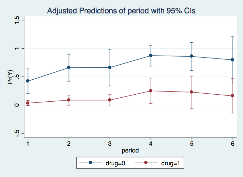
------------------------------------------------------------------------------Both drug and age are significant with the older patients more likely to die and those on drug therapy less likely. It can be useful to look at the hazard function to ascertain the effects over time. We will include both levels of drug while holding age at 56 (the median age). We will plot the results using marginsplot.
margins period, at(drug=(0 1) age=56)

Adjusted predictions                              Number of obs   =        143
Model VCE    : OIM

Expression   : Pr(y), predict()
1._at        : drug            =           0
               age             =          56
2._at        : drug            =           1
               age             =          56

------------------------------------------------------------------------------
             |            Delta-method
             |     Margin   Std. Err.      z    P>|z|     [95% Conf. Interval]
-------------+----------------------------------------------------------------
  _at#period |
        1 1  |   .4231272   .1101299     3.84   0.000     .2072766    .6389779
        1 2  |   .6602652   .1219254     5.42   0.000     .4212958    .8992346
        1 3  |   .6622139   .1655462     4.00   0.000     .3377493    .9866786
        1 4  |   .8730252   .0939619     9.29   0.000     .6888632    1.057187
        1 5  |   .8583836   .1268033     6.77   0.000     .6098536    1.106913
        1 6  |   .7985611   .2079556     3.84   0.000     .3909757    1.206147
        2 1  |    .034423    .022453     1.53   0.125    -.0095841    .0784301
        2 2  |   .0863077   .0455352     1.90   0.058    -.0029398    .1755551
        2 3  |   .0869962   .0530727     1.64   0.101    -.0170244    .1910167
        2 4  |   .2504758   .1150907     2.18   0.030     .0249023    .4760494
        2 5  |    .227563   .1452077     1.57   0.117    -.0570388    .5121648
        2 6  |   .1615519   .1546871     1.04   0.296    -.1416293     .464733
------------------------------------------------------------------------------

marginsplot, x(period)
Let's check the fit of this model. To do this we will rerun the model with a constant and then run the fitstat command. Notice that we have to drop one of the time dummies if we include the constant. Models without the constant but with all of the dummies and models with the constant dropping one dummy are equivalent they are merely different parameterizations of the same model.
quietly logit y i.drug age i.period

fitstat

Measures of Fit for logit of y

Log-Lik Intercept Only:        -74.761   Log-Lik Full Model:            -55.655
D(133):                        111.310   LR(7):                          38.213
                                         Prob > LR:                       0.000
McFadden's R2:                   0.256   McFadden's Adj R2:               0.122
ML (Cox-Snell) R2:               0.234   Cragg-Uhler(Nagelkerke) R2:      0.362
McKelvey & Zavoina's R2:         0.410   Efron's R2:                      0.271
Variance of y*:                  5.579   Variance of error:               3.290
Count R2:                        0.818   Adj Count R2:                    0.161
AIC:                             0.918   AIC*n:                         131.310
BIC:                          -548.748   BIC':                           -3.473
BIC used by Stata:             151.013   AIC used by Stata:             127.310
We can then compare the fit with a model that treats time as a continuous linear variable.
logit y i.drug age period

Iteration 0:   log likelihood = -74.761305
Iteration 1:   log likelihood = -58.627916
Iteration 2:   log likelihood = -56.804116
Iteration 3:   log likelihood = -56.782562
Iteration 4:   log likelihood = -56.782549
Iteration 5:   log likelihood = -56.782549

Logistic regression                               Number of obs   =        143
                                                  LR chi2(3)      =      35.96
                                                  Prob > chi2     =     0.0000
Log likelihood = -56.782549                       Pseudo R2       =     0.2405

------------------------------------------------------------------------------
           y |      Coef.   Std. Err.      z    P>|z|     [95% Conf. Interval]
-------------+----------------------------------------------------------------
      1.drug |  -2.903144   .6025594    -4.82   0.000    -4.084138   -1.722149
         age |   .1480103   .0495299     2.99   0.003     .0509336     .245087
      period |   .4508214   .1868348     2.41   0.016      .084632    .8170109
       _cons |  -8.849313   2.821481    -3.14   0.002    -14.37931   -3.319312
------------------------------------------------------------------------------

fitstat

Measures of Fit for logit of y

Log-Lik Intercept Only:        -74.761   Log-Lik Full Model:            -56.783
D(138):                        113.565   LR(3):                          35.958
                                         Prob > LR:                       0.000
McFadden's R2:                   0.240   McFadden's Adj R2:               0.174
ML (Cox-Snell) R2:               0.222   Cragg-Uhler(Nagelkerke) R2:      0.343
McKelvey & Zavoina's R2:         0.378   Efron's R2:                      0.262
Variance of y*:                  5.290   Variance of error:               3.290
Count R2:                        0.811   Adj Count R2:                    0.129
AIC:                             0.864   AIC*n:                         123.565
BIC:                          -571.307   BIC':                          -21.069
BIC used by Stata:             133.416   AIC used by Stata:             121.565
Based on the deviance (111.31 vs 113.565) and BIC (-558.674 vs -576.27) it appears that the model using indicator variables for time fits slightly better, although it uses four more degrees of freedom then the model with linear time.
Using a model that includes both period and k-2 dummy coded time variables indicates that the dummy coded time does not account for significantly more variability than using linear time alone.
logit y drug age i.period period

note: 6.period omitted because of collinearity
Iteration 0:   log likelihood = -74.761305
Iteration 1:   log likelihood = -57.764768
Iteration 2:   log likelihood =  -55.68916
Iteration 3:   log likelihood = -55.655082
Iteration 4:   log likelihood =  -55.65503
Iteration 5:   log likelihood =  -55.65503

Logistic regression                               Number of obs   =        143
                                                  LR chi2(7)      =      38.21
                                                  Prob > chi2     =     0.0000
Log likelihood =  -55.65503                       Pseudo R2       =     0.2556

------------------------------------------------------------------------------
           y |      Coef.   Std. Err.      z    P>|z|     [95% Conf. Interval]
-------------+----------------------------------------------------------------
        drug |  -3.024052   .6347087    -4.76   0.000    -4.268058   -1.780046
         age |   .1607128    .051414     3.13   0.002     .0599433    .2614823
      period |   .3374548   .2625646     1.29   0.199    -.1771623     .852072
             |
      period |
          2  |   .6369702   .6303464     1.01   0.312     -.598486    1.872426
          3  |   .3082149   .8214649     0.38   0.708    -1.301827    1.918257
          4  |    1.22556   .9543035     1.28   0.199    -.6448403    3.095961
          5  |   .7620581   1.241969     0.61   0.539    -1.672156    3.196272
          6  |          0  (omitted)
             |
       _cons |  -9.647322   2.979501    -3.24   0.001    -15.48704   -3.807607
------------------------------------------------------------------------------

testparm i.period

 ( 1)  [y]2.period = 0
 ( 2)  [y]3.period = 0
 ( 3)  [y]4.period = 0
 ( 4)  [y]5.period = 0

           chi2(  4) =    2.15
         Prob > chi2 =    0.7087
A Proportional Hazards ModelA discrete-time proportional hazards model can be estimated using the cloglog command.
cloglog y i.drug age ibn.period, nocons

Iteration 0:   log likelihood =   -58.5648
Iteration 1:   log likelihood = -55.720699
Iteration 2:   log likelihood = -55.701265
Iteration 3:   log likelihood = -55.701255
Iteration 4:   log likelihood = -55.701255

Complementary log-log regression                Number of obs     =        143
                                                Zero outcomes     =        112
                                                Nonzero outcomes  =         31

                                                Wald chi2(8)      =      51.91
Log likelihood = -55.701255                     Prob > chi2       =     0.0000

------------------------------------------------------------------------------
          _Y |      Coef.   Std. Err.      z    P>|z|     [95% Conf. Interval]
-------------+----------------------------------------------------------------
        drug |  -2.460096   .4880544    -5.04   0.000    -3.416665   -1.503527
         age |   .1273736    .040619     3.14   0.002     .0477619    .2069853
         _d1 |  -7.770962   2.354981    -3.30   0.001    -12.38664   -3.155284
         _d2 |  -7.085621   2.266325    -3.13   0.002    -11.52754   -2.643705
         _d3 |  -7.077778   2.277786    -3.11   0.002    -11.54216   -2.613399
         _d4 |  -5.956626   2.250857    -2.65   0.008    -10.36822   -1.545026
         _d5 |  -6.079785   2.342926    -2.59   0.009    -10.67183   -1.487735
         _d6 |  -6.377616   2.474713    -2.58   0.010    -11.22796   -1.527268
------------------------------------------------------------------------------

glm y i.drug age ibn.period, fam(bin) link(clog) nocons

Iteration 0:   log likelihood = -60.789135
Iteration 1:   log likelihood = -55.756479
Iteration 2:   log likelihood = -55.701292
Iteration 3:   log likelihood = -55.701255
Iteration 4:   log likelihood = -55.701255

Generalized linear models                          No. of obs      =       143
Optimization     : ML                              Residual df     =       135
                                                   Scale parameter =         1
Deviance         =  111.4025091                    (1/df) Deviance =  .8252038
Pearson          =  132.6671546                    (1/df) Pearson  =  .9827197

Variance function: V(u) = u*(1-u)                  [Bernoulli]
Link function    : g(u) = ln(-ln(1-u))             [Complementary log-log]

                                                   AIC             =  .8909266
Log likelihood   = -55.70125456                    BIC             = -558.5815

------------------------------------------------------------------------------
             |                 OIM
           y |      Coef.   Std. Err.      z    P>|z|     [95% Conf. Interval]
-------------+----------------------------------------------------------------
      1.drug |  -2.460096   .4880544    -5.04   0.000    -3.416665   -1.503527
         age |   .1273736    .040619     3.14   0.002     .0477619    .2069853
             |
      period |
          1  |  -7.770962   2.354981    -3.30   0.001    -12.38664   -3.155284
          2  |  -7.085621   2.266325    -3.13   0.002    -11.52754   -2.643705
          3  |  -7.077778   2.277786    -3.11   0.002    -11.54216   -2.613399
          4  |  -5.956626   2.250857    -2.65   0.008    -10.36822   -1.545026
          5  |  -6.079785   2.342926    -2.59   0.009    -10.67183   -1.487735
          6  |  -6.377616   2.474713    -2.58   0.010    -11.22796   -1.527268
------------------------------------------------------------------------------

glm, eform noheader

------------------------------------------------------------------------------
             |                 OIM
           y |     exp(b)   Std. Err.      z    P>|z|     [95% Conf. Interval]
-------------+----------------------------------------------------------------
      1.drug |   .0854267   .0416929    -5.04   0.000     .0328217    .2223446
         age |   1.135841   .0461367     3.14   0.002     1.048921    1.229964
             |
      period |
          1  |   .0004218   .0009933    -3.30   0.001     4.17e-06    .0426263
          2  |   .0008371    .001897    -3.13   0.002     9.85e-06    .0710974
          3  |   .0008436   .0019216    -3.11   0.002     9.71e-06     .073285
          4  |   .0025886   .0058266    -2.65   0.008     .0000314    .2133062
          5  |   .0022887   .0053622    -2.59   0.009     .0000232    .2258837
          6  |   .0016992    .004205    -2.58   0.010     .0000133    .2171281
------------------------------------------------------------------------------
There is also a program called pgmhaz (findit pgmhaz) that esitmates two
different discrete time proportional
hazards models, one of which incorporates a
gamma mixture distribution to summarize unobserved individual
heterogeneity (or "frailty").
tab period, gen(p)

pgmhaz drug age p1-p6, id(id) seq(period) dead(y) nocons

(1) PGM hazard model without unobserved heterogeneity

Iteration 1 : deviance =  121.5783
Iteration 2 : deviance =  111.9325
Iteration 3 : deviance =  111.4106
Iteration 4 : deviance =  111.4026
Iteration 5 : deviance =  111.4025
Iteration 6 : deviance =  111.4025

Residual df  =       135                                No. of obs =       143
Pearson X2   =  132.6589                                Deviance   =  111.4025
Dispersion   =  .9826588                                Dispersion =  .8252038

Bernoulli distribution, cloglog link
------------------------------------------------------------------------------
           y |      Coef.   Std. Err.      z    P>|z|     [95% Conf. Interval]
-------------+----------------------------------------------------------------
        drug |  -2.460075   .4854314    -5.07   0.000    -3.411503   -1.508647
         age |   .1273721   .0395082     3.22   0.001     .0499374    .2048068
          p1 |  -7.770891   2.310665    -3.36   0.001    -12.29971   -3.242069
          p2 |  -7.085539    2.18251    -3.25   0.001    -11.36318   -2.807897
          p3 |  -7.077696   2.209682    -3.20   0.001    -11.40859   -2.746799
          p4 |  -5.956576   2.168435    -2.75   0.006    -10.20663   -1.706522
          p5 |  -6.079717   2.260327    -2.69   0.007    -10.50988   -1.649557
          p6 |  -6.377553   2.405179    -2.65   0.008    -11.09162   -1.663489
------------------------------------------------------------------------------
Log likelihood (-0.5*Deviance) = -55.701255
   Cf. log likelihood for intercept-only model (Model 0) = -74.761305
   Chi-squared statistic for Model (1) vs. Model (0) = 38.120101
   Prob. > chi2(7) = 2.875e-06

(2) PGM hazard model with Gamma distributed unobserved heterogeneity

Iteration 0:  Log Likelihood = -56.479417
Iteration 1:  Log Likelihood = -55.499011
Iteration 2:  Log Likelihood = -55.487301
Iteration 3:  Log Likelihood = -55.486459
Iteration 4:  Log Likelihood = -55.486458
Iteration 5:  Log Likelihood = -55.486458

PGM hazard model with Gamma heterogeneity           Number of obs    =     143
                                                    Model chi2(8)    =       .
                                                    Prob > chi2      =       .
Log Likelihood =    -55.4864576

------------------------------------------------------------------------------
           y |      Coef.   Std. Err.      z    P>|z|     [95% Conf. Interval]
-------------+----------------------------------------------------------------
hazard       |
        drug |   -2.96652   1.000101    -2.97   0.003    -4.926683   -1.006358
         age |   .1574424   .0688266     2.29   0.022     .0225448      .29234
          p1 |    -9.2916   3.703829    -2.51   0.012    -16.55097   -2.032227
          p2 |  -8.306118   3.325504    -2.50   0.013    -14.82399    -1.78825
          p3 |  -8.129395   3.189787    -2.55   0.011    -14.38126   -1.877528
          p4 |   -6.90202   3.039796    -2.27   0.023    -12.85991   -.9441291
          p5 |  -6.970558   3.035029    -2.30   0.022    -12.91911   -1.022011
          p6 |  -7.160582   3.054765    -2.34   0.019    -13.14781   -1.173351
-------------+----------------------------------------------------------------
ln_varg      |
       _cons |  -.9778872   1.690062    -0.58   0.563    -4.290347    2.334573
------------------------------------------------------------------------------
Gamma variance, exp(ln_varg) = .3761049; Std. Err. = .63564044; z = .59169441

Likelihood ratio statistic for testing models (1) vs (2) = .42959389
Prob. test statistic > chi2(1) = .51218829

pgmhaz, eform

PGM hazard model with Gamma heterogeneity           Number of obs    =     143
                                                    Model chi2(8)    =       .
                                                    Prob > chi2      =       .
Log Likelihood =    -55.4864576

------------------------------------------------------------------------------
           y |          :   Std. Err.      z    P>|z|     [95% Conf. Interval]
-------------+----------------------------------------------------------------
hazard       |
        drug |   .0514821   .0514874    -2.97   0.003     .0072505     .365548
         age |   1.170513   .0805624     2.29   0.022     1.022801    1.339558
          p1 |   .0000922   .0003415    -2.51   0.012     6.49e-08    .1310433
          p2 |    .000247   .0008214    -2.50   0.013     3.65e-07    .1672527
          p3 |   .0002947   .0009402    -2.55   0.011     5.68e-07    .1529678
          p4 |   .0010058   .0030573    -2.27   0.023     2.60e-06    .3890182
          p5 |   .0009391   .0028503    -2.30   0.022     2.45e-06    .3598707
          p6 |   .0007766   .0023723    -2.34   0.019     1.95e-06    .3093285
-------------+----------------------------------------------------------------
ln_varg      |
------------------------------------------------------------------------------
Gamma variance, exp(ln_varg) = .3761049; Std. Err. = .63564044; z = .59169441

Likelihood ratio statistic for testing models (1) vs (2) = .42959389
Prob. test statistic > chi2(1) = .51218829
Categorical Data Analysis Course
Phil Ender