
Item response models may be used to model the responses of subjects to a number of questions or test items. An item response model with one parameter for item difficulty is known as a Rasch model. Georg Rasch (1901-1980), a Danish statistician, gave an axiomatic derivation of the model in the 1960s. We will be using a conditional (fixed-effects) logit model to illustrate the model, however, Rasch's derivation used a different approach, but one that turns out to be equivalent to the fixed-effects logit. Rasch models are one of the dominant models for binary items (e.g., success/failure on test items) in psychometrics.
In the Rasch model the log odds of subject i giving a correct response to item j may be modeled using a one-parameter logistic response model
In terms of probability the model looks like this,
Example
use http://www.gseis.ucla.edu/courses/data/lsat3

listblck in 51/65

            id       item       resp        i1        i2        i3        i4        i5      total
 51.      3002          1          0        -1         0         0         0         0          1
 52.      3002          2          0         0        -1         0         0         0          1
 53.      3002          3          0         0         0        -1         0         0          1
 54.      3002          4          1         0         0         0        -1         0          1
 55.      3002          5          0         0         0         0         0        -1          1
 56.      4001          1          0        -1         0         0         0         0          2
 57.      4001          2          0         0        -1         0         0         0          2
 58.      4001          3          0         0         0        -1         0         0          2
 59.      4001          4          1         0         0         0        -1         0          2
 60.      4001          5          1         0         0         0         0        -1          2
 61.      4002          1          0        -1         0         0         0         0          2
 62.      4002          2          0         0        -1         0         0         0          2
 63.      4002          3          0         0         0        -1         0         0          2
 64.      4002          4          1         0         0         0        -1         0          2
 65.      4002          5          1         0         0         0         0        -1          2

tabulate total if item==1

      total |      Freq.     Percent        Cum.
------------+-----------------------------------
          0 |          3        0.30        0.30
          1 |         20        2.00        2.30
          2 |         85        8.50       10.80
          3 |        237       23.70       34.50
          4 |        357       35.70       70.20
          5 |        298       29.80      100.00
------------+-----------------------------------
      Total |       1000      100.00

tabulate item resp, row nofreq

           |         resp
      item |         0          1 |     Total
-----------+----------------------+----------
         1 |      7.60      92.40 |    100.00
         2 |     29.10      70.90 |    100.00
         3 |     44.70      55.30 |    100.00
         4 |     23.70      76.30 |    100.00
         5 |     13.00      87.00 |    100.00
-----------+----------------------+----------
     Total |     23.62      76.38 |    100.00
Item 1 is the easiest item, responded correctly by the
most subjects, so we will use it as the reference item. We will run an fixed-effects xtlogit
using the negative indicators for each of the remaining items. The fixed effects xtlogit is
equivalent to running the conditional logistic command clogit.
xtlogit resp i2 i3 i4 i5, i(id) fe
/* clogit resp i2 i3 i4 i5, group(id)  */

note: multiple positive outcomes within groups encountered.
note: 301 groups (1505 obs) dropped due to all positive or
      all negative outcomes.

Conditional fixed-effects logit                 Number of obs      =      3495
Group variable (i) : id                         Number of groups   =       699

                                                Obs per group: min =         5
                                                               avg =       5.0
                                                               max =         5

                                                LR chi2(4)         =    513.24
Log likelihood  = -1091.5697                    Prob > chi2        =    0.0000

------------------------------------------------------------------------------
        resp |      Coef.   Std. Err.      z    P>|z|     [95% Conf. Interval]
-------------+----------------------------------------------------------------
          i2 |   1.731034   .1446523    11.97   0.000     1.447521    2.014548
          i3 |   2.492113   .1441542    17.29   0.000     2.209576     2.77465
          i4 |   1.424539    .146451     9.73   0.000       1.1375    1.711578
          i5 |   .6329562   .1566198     4.04   0.000     .3259869    .9399254
------------------------------------------------------------------------------
Item 1, the easiest item, has a difficulty value fixed at zero. Item 3 is the most difficult
item with a coefficient of 2.49. Note that the fixed-effects xtlogit has
dropped 301 subjects from the analysis. These subjects either responded to all items correctly
or to all items incorrectly; in a conditional likelihood these subjects carry no information
about the difficulty of the items.We can also look at the item difficulty in terms of the probability of getting an items correct.
predict p1
(option pc1 assumed; conditional probability for single outcome within group)

tablist item p1     /* available from ATS */

  +------------------------+
  | item         p1   Freq |
  |------------------------|
  |    1   .4922531   1000 |
  |    2   .0871786   1000 |
  |    3   .0407266   1000 |
  |    4   .1184456   1000 |
  |    5   .2613961   1000 |
  +------------------------+
Looking at the item probabilities, we see that Item 1 has the highest probability (P = .49) of a correct response and Item 3 has the lowest probability (P = .04) of a correct response. The probabilities follow the same difficulty patterns and the coefficients.
We can check our model specification that the difficulty parameters are the same for the "poor" (low scoring) subjects and the "good" (high scoring) subjects, distinguished by their total score. We will do this using Hausman tests versus low scoring subjects (total = 0,1 or 2) and versus high scoring subjects (total = 3,4 or 5). The hausman command with the less option compares the fully efficient model with the less efficient, but consistent model.
hausman, save

xtlogit resp i2 i3 i4 i5 if total<3, i(id) fe nolog
note: multiple positive outcomes within groups encountered.
note: 3 groups (15 obs) dropped due to all positive or
      all negative outcomes.

Conditional fixed-effects logit                 Number of obs      =       525
Group variable (i) : id                         Number of groups   =       105

                                                Obs per group: min =         5
                                                               avg =       5.0
                                                               max =         5

                                                LR chi2(4)         =     93.26
Log likelihood  = -181.27655                    Prob > chi2        =    0.0000

------------------------------------------------------------------------------
        resp |      Coef.   Std. Err.      z    P>|z|     [95% Conf. Interval]
-------------+----------------------------------------------------------------
          i2 |   1.533091    .279329     5.49   0.000     .9856159    2.080566
          i3 |   2.743066   .4007517     6.84   0.000     1.957607    3.528525
          i4 |   1.326592   .2689439     4.93   0.000     .7994716    1.853712
          i5 |   .5548602   .2587489     2.14   0.032     .0477217    1.061999
------------------------------------------------------------------------------

hausman, less

                ---- Coefficients ----
             |      (b)          (B)            (b-B)   sqrt(diag(V_b-V_B))
             |    Current       Prior        Difference        S.E.
-------------+-------------------------------------------------------------
          i2 |   1.533091     1.731034        -.1979437     .2389569
          i3 |   2.743066     2.492113         .2509529     .3739272
          i4 |   1.326592     1.424539         -.097947     .2255725
          i5 |   .5548602     .6329562         -.078096     .2059641
---------------------------------------------------------------------------
                b = less efficient estimates obtained from clogit
                B = fully efficient estimates obtained previously from clogit

    Test:  Ho:  difference in coefficients not systematic

                chi2(  4) = (b-B)'[(V_b-V_B)^(-1)](b-B)
                          =     1.50
                          Prob>chi2 =     0.8275

xtlogit resp i2 i3 i4 i5 if total>2, i(id) fe nolog
note: multiple positive outcomes within groups encountered.
note: 298 groups (1490 obs) dropped due to all positive or
      all negative outcomes.

Conditional fixed-effects logit                 Number of obs      =      2970
Group variable (i) : id                         Number of groups   =       594

                                                Obs per group: min =         5
                                                               avg =       5.0
                                                               max =         5

                                                LR chi2(4)         =    421.53
Log likelihood  =   -909.517                    Prob > chi2        =    0.0000

------------------------------------------------------------------------------
        resp |      Coef.   Std. Err.      z    P>|z|     [95% Conf. Interval]
-------------+----------------------------------------------------------------
          i2 |   1.789893   .1775602    10.08   0.000     1.441881    2.137904
          i3 |   2.519253   .1748241    14.41   0.000     2.176604    2.861902
          i4 |   1.472984   .1812922     8.12   0.000     1.117658     1.82831
          i5 |   .6810296   .1984919     3.43   0.001     .2919926    1.070067
------------------------------------------------------------------------------

hausman, less

                ---- Coefficients ----
             |      (b)          (B)            (b-B)   sqrt(diag(V_b-V_B))
             |    Current       Prior        Difference        S.E.
-------------+-------------------------------------------------------------
          i2 |   1.789893     1.731034         .0588582     .1029725
          i3 |   2.519253     2.492113         .0271404     .0989092
          i4 |   1.472984     1.424539         .0484448     .1068596
          i5 |   .6810296     .6329562         .0480734     .1219396
---------------------------------------------------------------------------
                b = less efficient estimates obtained from clogit
                B = fully efficient estimates obtained previously from clogit

    Test:  Ho:  difference in coefficients not systematic

                chi2(  4) = (b-B)'[(V_b-V_B)^(-1)](b-B)
                          =     1.59
                          Prob>chi2 =     0.8097
Rasch models, along with other item response models, have an assumption of local independence,
that is, the responses to a given item are independent of the responses to other items in
the test. In practical terms, this implies Pr(yij=1 & yik=1) =
Pr(yij=1)*Pr(yik=1).
Further, Rasch models, because they are one-parameter models, assume that all of the items
have equal discrimination, that is, the items discriminate equally well for "good" subjects as
they do for "poor" subjects. Two-parameter and three-parameter item response models include measures
of item discrimination along with item difficulty.It is also possible to estimate the model using the gllamm command. gllamm is short for generalized linear latent and mixed models. This is, in fact, a random effects model. Note that the model includes a constant.
gllamm resp i2 i3 i4 i5, i(id) fam(binom) link(logit)

Iteration 0:   log likelihood = -2474.5358
Iteration 1:   log likelihood = -2467.6634
Iteration 2:   log likelihood = -2466.9383
Iteration 3:   log likelihood = -2466.9377
Iteration 4:   log likelihood = -2466.9377

number of level 1 units = 5000
number of level 2 units = 1000

Condition Number = 7.5146066

gllamm model

log likelihood = -2466.9377

------------------------------------------------------------------------------
        resp |      Coef.   Std. Err.      z    P>|z|     [95% Conf. Interval]
-------------+----------------------------------------------------------------
          i2 |    1.73141   .1440341    12.02   0.000     1.449108    2.013712
          i3 |   2.490159   .1437773    17.32   0.000     2.208361    2.771958
          i4 |   1.423565   .1457916     9.76   0.000     1.137818    1.709311
          i5 |   .6306089   .1561066     4.04   0.000     .3246455    .9365723
       _cons |   2.730011   .1304411    20.93   0.000     2.474351    2.985671
------------------------------------------------------------------------------


Variances and covariances of random effects
------------------------------------------------------------------------------


***level 2 (id)

    var(1): .57022578 (.10486574)
One advantage to using gllamm is that we can include all of
the items by specifying the nocons option.
gllamm resp i1 i2 i3 i4 i5, i(id) fam(binom) link(logit) nolog nocons

number of level 1 units = 5000
number of level 2 units = 1000

Condition Number = 2.3631559

gllamm model

log likelihood = -2466.9377

------------------------------------------------------------------------------
        resp |      Coef.   Std. Err.      z    P>|z|     [95% Conf. Interval]
-------------+----------------------------------------------------------------
          i1 |  -2.730012   .1304412   -20.93   0.000    -2.985672   -2.474352
          i2 |  -.9986011   .0791763   -12.61   0.000    -1.153784   -.8434185
          i3 |  -.2398516   .0717745    -3.34   0.001     -.380527   -.0991762
          i4 |  -1.306446   .0846371   -15.44   0.000    -1.472332   -1.140561
          i5 |  -2.099402   .1054448   -19.91   0.000     -2.30607   -1.892734
------------------------------------------------------------------------------


Variances and covariances of random effects
------------------------------------------------------------------------------


***level 2 (id)

    var(1): .57022593 (.10486576)
------------------------------------------------------------------------------
Now we can compute the conditional probabilities using gllapred.
generate e1=-2.730012
generate e2=-.9986011
generate e3=-.2398516
generate e4=-1.306446
generate e5=-2.099402

gllapred, cp, mu us(e)

tablist item cp p1

  +------------------------------------+
  | item          cp         p1   Freq |
  |------------------------------------|
  |    1   .49999993   .4922531   1000 |
  |    2   .15040721   .0871786   1000 |
  |    3   .07655087   .0407266   1000 |
  |    4   .19410324   .1184456   1000 |
  |    5   .34737228   .2613961   1000 |
  +------------------------------------+
use http://www.gseis.ucla.edu/courses/data/lsat0

list in 1/30

     +----------------------------------------------+
     |   id   resp1   resp2   resp3   resp4   resp5 |
     |----------------------------------------------|
  1. | 1001       0       0       0       0       0 |
  2. | 1002       0       0       0       0       0 |
  3. | 1003       0       0       0       0       0 |
  4. | 2001       0       0       0       0       1 |
  5. | 2002       0       0       0       0       1 |
     |----------------------------------------------|
  6. | 2003       0       0       0       0       1 |
  7. | 2004       0       0       0       0       1 |
  8. | 2005       0       0       0       0       1 |
  9. | 2006       0       0       0       0       1 |
 10. | 3001       0       0       0       1       0 |
     |----------------------------------------------|
 11. | 3002       0       0       0       1       0 |
 12. | 4001       0       0       0       1       1 |
 13. | 4002       0       0       0       1       1 |
 14. | 4003       0       0       0       1       1 |
 15. | 4004       0       0       0       1       1 |
     |----------------------------------------------|
 16. | 4005       0       0       0       1       1 |
 17. | 4006       0       0       0       1       1 |
 18. | 4007       0       0       0       1       1 |
 19. | 4008       0       0       0       1       1 |
 20. | 4009       0       0       0       1       1 |
     |----------------------------------------------|
 21. | 4010       0       0       0       1       1 |
 22. | 4011       0       0       0       1       1 |
 23. | 5001       0       0       1       0       0 |
 24. | 6001       0       0       1       0       1 |
 25. | 7001       0       0       1       1       0 |
     |----------------------------------------------|
 26. | 7002       0       0       1       1       0 |
 27. | 7003       0       0       1       1       0 |
 28. | 8001       0       0       1       1       1 |
 29. | 8002       0       0       1       1       1 |
 30. | 8003       0       0       1       1       1 |
     +----------------------------------------------+

generate total=resp1+resp2+resp3+resp4+resp5

list in 1/30

     +------------------------------------------------------+
     |   id   resp1   resp2   resp3   resp4   resp5   total |
     |------------------------------------------------------|
  1. | 1001       0       0       0       0       0       0 |
  2. | 1002       0       0       0       0       0       0 |
  3. | 1003       0       0       0       0       0       0 |
  4. | 2001       0       0       0       0       1       1 |
  5. | 2002       0       0       0       0       1       1 |
     |------------------------------------------------------|
  6. | 2003       0       0       0       0       1       1 |
  7. | 2004       0       0       0       0       1       1 |
  8. | 2005       0       0       0       0       1       1 |
  9. | 2006       0       0       0       0       1       1 |
 10. | 3001       0       0       0       1       0       1 |
     |------------------------------------------------------|
 11. | 3002       0       0       0       1       0       1 |
 12. | 4001       0       0       0       1       1       2 |
 13. | 4002       0       0       0       1       1       2 |
 14. | 4003       0       0       0       1       1       2 |
 15. | 4004       0       0       0       1       1       2 |
     |------------------------------------------------------|
 16. | 4005       0       0       0       1       1       2 |
 17. | 4006       0       0       0       1       1       2 |
 18. | 4007       0       0       0       1       1       2 |
 19. | 4008       0       0       0       1       1       2 |
 20. | 4009       0       0       0       1       1       2 |
     |------------------------------------------------------|
 21. | 4010       0       0       0       1       1       2 |
 22. | 4011       0       0       0       1       1       2 |
 23. | 5001       0       0       1       0       0       1 |
 24. | 6001       0       0       1       0       1       2 |
 25. | 7001       0       0       1       1       0       2 |
     |------------------------------------------------------|
 26. | 7002       0       0       1       1       0       2 |
 27. | 7003       0       0       1       1       0       2 |
 28. | 8001       0       0       1       1       1       3 |
 29. | 8002       0       0       1       1       1       3 |
 30. | 8003       0       0       1       1       1       3 |
     +------------------------------------------------------+

reshape long resp, i(id) j(item)

list in 46/65

     +----------------------------+
     |   id   item   resp   total |
     |----------------------------|
 46. | 3001      1      0       1 |
 47. | 3001      2      0       1 |
 48. | 3001      3      0       1 |
 49. | 3001      4      1       1 |
 50. | 3001      5      0       1 |
     |----------------------------|
 51. | 3002      1      0       1 |
 52. | 3002      2      0       1 |
 53. | 3002      3      0       1 |
 54. | 3002      4      1       1 |
 55. | 3002      5      0       1 |
     |----------------------------|
 56. | 4001      1      0       2 |
 57. | 4001      2      0       2 |
 58. | 4001      3      0       2 |
 59. | 4001      4      1       2 |
 60. | 4001      5      1       2 |
     |----------------------------|
 61. | 4002      1      0       2 |
 62. | 4002      2      0       2 |
 63. | 4002      3      0       2 |
 64. | 4002      4      1       2 |
 65. | 4002      5      1       2 |
     +----------------------------+

for num 1/5 : gen iX = -(X==item)

list in 1/30

     +-----------------------------------------------------+
     |   id   item   resp   total   i1   i2   i3   i4   i5 |
     |-----------------------------------------------------|
  1. | 1001      1      0       0   -1    0    0    0    0 |
  2. | 1001      2      0       0    0   -1    0    0    0 |
  3. | 1001      3      0       0    0    0   -1    0    0 |
  4. | 1001      4      0       0    0    0    0   -1    0 |
  5. | 1001      5      0       0    0    0    0    0   -1 |
     |-----------------------------------------------------|
  6. | 1002      1      0       0   -1    0    0    0    0 |
  7. | 1002      2      0       0    0   -1    0    0    0 |
  8. | 1002      3      0       0    0    0   -1    0    0 |
  9. | 1002      4      0       0    0    0    0   -1    0 |
 10. | 1002      5      0       0    0    0    0    0   -1 |
     |-----------------------------------------------------|
 11. | 1003      1      0       0   -1    0    0    0    0 |
 12. | 1003      2      0       0    0   -1    0    0    0 |
 13. | 1003      3      0       0    0    0   -1    0    0 |
 14. | 1003      4      0       0    0    0    0   -1    0 |
 15. | 1003      5      0       0    0    0    0    0   -1 |
     |-----------------------------------------------------|
 16. | 2001      1      0       1   -1    0    0    0    0 |
 17. | 2001      2      0       1    0   -1    0    0    0 |
 18. | 2001      3      0       1    0    0   -1    0    0 |
 19. | 2001      4      0       1    0    0    0   -1    0 |
 20. | 2001      5      1       1    0    0    0    0   -1 |
     |-----------------------------------------------------|
 21. | 2002      1      0       1   -1    0    0    0    0 |
 22. | 2002      2      0       1    0   -1    0    0    0 |
 23. | 2002      3      0       1    0    0   -1    0    0 |
 24. | 2002      4      0       1    0    0    0   -1    0 |
 25. | 2002      5      1       1    0    0    0    0   -1 |
     |-----------------------------------------------------|
 26. | 2003      1      0       1   -1    0    0    0    0 |
 27. | 2003      2      0       1    0   -1    0    0    0 |
 28. | 2003      3      0       1    0    0   -1    0    0 |
 29. | 2003      4      0       1    0    0    0   -1    0 |
 30. | 2003      5      1       1    0    0    0    0   -1 |
     +-----------------------------------------------------+
A Stata Program: raschtestJean-Benoit Hardouin of the Regional Health Observatory in France has written several ado programs that will perform a maximum likelihood Rasch analysis. You will need the ado files raschtest.ado and gammasym.ado. The example below uses version 7.3 of raschtest dated 2july2005.
The data are organized differently from the analysis above. The data are organized by individual with each item scored right or wrong (0 or 1). We will use the dataset lsat3 reshaping it to the proper form.
use http://www.gseis.ucla.edu/courses/data/lsat3, clear

drop i1- total
rename item q
rename resp item
reshape wide item, i(id) j(q)

list in 1/20, clean

         id   item1   item2   item3   item4   item5
  1.   1001       0       0       0       0       0
  2.   1002       0       0       0       0       0
  3.   1003       0       0       0       0       0
  4.   2001       0       0       0       0       1
  5.   2002       0       0       0       0       1
  6.   2003       0       0       0       0       1
  7.   2004       0       0       0       0       1
  8.   2005       0       0       0       0       1
  9.   2006       0       0       0       0       1
 10.   3001       0       0       0       1       0
 11.   3002       0       0       0       1       0
 12.   4001       0       0       0       1       1
 13.   4002       0       0       0       1       1
 14.   4003       0       0       0       1       1
 15.   4004       0       0       0       1       1
 16.   4005       0       0       0       1       1
 17.   4006       0       0       0       1       1
 18.   4007       0       0       0       1       1
 19.   4008       0       0       0       1       1
 20.   4009       0       0       0       1       1
The raschtest program computes both the item difficulties and the ability parameters.
raschtest item1-item5

Estimation method: Conditional maximum likelihood (CML)
Number of items: 5
Number of groups: 6 (4 of them are used to compute the statistics of test)
Number of individuals: 1000 (0 individuals removed for missing values)
Number of individuals with nul or perfect score: 301
Conditional log-likelihood: -1091.5697
Log-likelihood: -1849.5149

               Difficulty                                Standardized
        Items  parameters  std Err.     R1c   df p-value Outfit  Infit      U
-----------------------------------------------------------------------------
         item1   -0.63296   0.15662   0.217    3  0.9749 -0.026 -0.081  0.116
         item2    1.09808   0.12276   1.555    3  0.6696 -0.085  0.065 -0.193
         item3    1.85916   0.12182   0.910    3  0.8231 -0.415 -0.346 -0.340
         item4    0.79158   0.12508   0.198    3  0.9779  0.115  0.165  0.117
        item5*    0.00000        .    0.119    3  0.9894  0.141  0.140  0.281
-----------------------------------------------------------------------------
     R1c test                  R1c=   3.012   12  0.9955
     Andersen LR test            Z=   3.136   12  0.9945
-----------------------------------------------------------------------------
*: The difficulty parameter of this item had been fixed to 0
You have groups of scores with less than 30 individuals. The tests can be invalid.


                                Ability                    Expected
                Group Score  parameters  std Err.    Freq.    Score       ll
                --------------------------------------------------------------
                    0     0      -2.167     2.790        3     0.38
                --------------------------------------------------------------
                    1     1      -0.714     0.735       20     1.20   -24.7519
                --------------------------------------------------------------
                    2     2       0.212     0.483       85     2.06  -155.9384
                --------------------------------------------------------------
                    3     3       1.045     0.479      237     2.94  -437.7270
                --------------------------------------------------------------
                    4     4       1.959     0.727      357     3.80  -471.5843
                --------------------------------------------------------------
                    5     5       3.400     2.763      298     4.61
                --------------------------------------------------------------
By default, raschtest sets the difficulty of the last item in the list to zero,
so the values of the difficulty parameters are different in this analysis. But note that item1
is the easiest item. We can make item1 have a difficulty of zero by changing the order of
the variables in the command so that item1 comes last. Now the items difficulties are the
same as in our original xtlogit (conditional logistic) example. The
genlt option generates latent trait (ability) scores for each subject and the genscore
option gives a total correct for each observation.
raschtest item2-item5 item1, genlt(ltscore) genscore(totscore)
Estimation method: Conditional maximum likelihood (CML)
Number of items: 5
Number of groups: 6 (4 of them are used to compute the statistics of test)
Number of individuals: 1000 (0 individuals removed for missing values)
Number of individuals with nul or perfect score: 301
Conditional log-likelihood: -1091.5697
Log-likelihood: -1849.5066
Difficulty Standardized
Items parameters std Err. R1c df p-value Outfit Infit U
-----------------------------------------------------------------------------
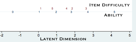
item2 1.73103 0.14465 1.350 3 0.7173 -0.085 0.065 -0.193
item3 2.49211 0.14415 1.025 3 0.7951 -0.415 -0.346 -0.340
item4 1.42454 0.14645 0.145 3 0.9859 0.115 0.165 0.117
item5 0.63296 0.15662 0.147 3 0.9856 0.141 0.140 0.281
item1* 0.00000 . 0.204 3 0.9770 -0.026 -0.081 0.116
-----------------------------------------------------------------------------
R1c test R1c= 3.012 12 0.9955
Andersen LR test Z= 3.136 12 0.9945
-----------------------------------------------------------------------------
*: The difficulty parameter of this item had been fixed to 0
You have groups of scores with less than 30 individuals. The tests can be invalid.
Ability Expected
Group Score parameters std Err. Freq. Score ll
--------------------------------------------------------------
0 0 -1.534 2.790 3 0.38
--------------------------------------------------------------
1 1 -0.081 0.735 20 1.20 -24.7519
--------------------------------------------------------------
2 2 0.845 0.483 85 2.06 -155.9384
--------------------------------------------------------------
3 3 1.678 0.479 237 2.94 -437.7270
--------------------------------------------------------------
4 4 2.592 0.727 357 3.80 -471.5843
--------------------------------------------------------------
5 5 4.033 2.763 298 4.61
--------------------------------------------------------------
We can graph both item difficulty and ability on the same latent dimension.
list in 1/20, clean

         id   item1   item2   item3   item4   item5   totscore   ltscore
  1.   1001       0       0       0       0       0          0    -1.534
  2.   1002       0       0       0       0       0          0    -1.534
  3.   1003       0       0       0       0       0          0    -1.534
  4.   2001       0       0       0       0       1          1     -.081
  5.   2002       0       0       0       0       1          1     -.081
  6.   2003       0       0       0       0       1          1     -.081
  7.   2004       0       0       0       0       1          1     -.081
  8.   2005       0       0       0       0       1          1     -.081
  9.   2006       0       0       0       0       1          1     -.081
 10.   3001       0       0       0       1       0          1     -.081
 11.   3002       0       0       0       1       0          1     -.081
 12.   4001       0       0       0       1       1          2      .845
 13.   4002       0       0       0       1       1          2      .845
 14.   4003       0       0       0       1       1          2      .845
 15.   4004       0       0       0       1       1          2      .845
 16.   4005       0       0       0       1       1          2      .845
 17.   4006       0       0       0       1       1          2      .845
 18.   4007       0       0       0       1       1          2      .845
 19.   4008       0       0       0       1       1          2      .845
 20.   4009       0       0       0       1       1          2      .845
Categorical Data Analysis Course
Phil Ender revised 21feb06