Correspondence analysis represents yet one more method for analyzing data in contingency tables. Correspondence analysis was developed in France and is more commonly used in Europe than in North America. Correspondence analysis is a descriptive/exploratory technique designed to analyze two-way and multi-way tables containing measures of correspondence between the row and column variables. The results produced by correspondence analysis provide information which is similar to that produced by principal components or factor analysis. They allow one to explore the structure of the categorical variables included in the table.
Correspondence analysis seeks to represent the relationships among the categories of row and column variables with a smaller number of latent dimensions. It produces a graphical representation of the relationships between the row and column categories in the same space.
We will illustrate correspondence analysis using the ca command (new in Stata 9) with the hsb2 dataset. In looking at the relationship between race and ses there can be at most two dimensions. The maximum number of dimensions is the minimum(R-1, C-1). Since ses has three categories, C-1 = 2. In this example, as you will see, the first dimension accounts for about 98% of the variability, so there is really only one dimension.
Some terminology: Mass is just the relative frequencies for each of the marginal categorites. The total inertia is the chi-square value divided by N. It is partioned into parts for each of the dimensions. We can write inertia as the weighted sum of the chi-square distance between each profile and the mean profile.
Example 1
use http://www.gseis.ucla.edu/courses/data/hsb2,clear
tabulate race ses, chi2
| ses
race | low middle high | Total
-------------+---------------------------------+----------
hispanic | 9 11 4 | 24
asian | 3 5 3 | 11
african-amer | 11 6 3 | 20
white | 24 73 48 | 145
-------------+---------------------------------+----------
Total | 47 95 58 | 200
Pearson chi2(6) = 18.5160 Pr = 0.005
/* row profile */
tabulate race ses, row nofreq
| ses
race | low middle high | Total
-------------+---------------------------------+----------
hispanic | 37.50 45.83 16.67 | 100.00
asian | 27.27 45.45 27.27 | 100.00
african-amer | 55.00 30.00 15.00 | 100.00
white | 16.55 50.34 33.10 | 100.00
-------------+---------------------------------+----------
Total | 23.50 47.50 29.00 | 100.00
/* code to plot row profiles */
preserve
contract race ses
sort race
by race: gen rsum = sum(_freq)
by race: gen rpro = _freq/rsum[_N]
drop _freq rsum
reshape wide rpro, i(race) j(ses)
/* findit triplot */
triplot rpro1 rpro2 rpro3
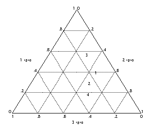 restore
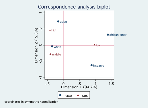
ca race ses,
Correspondence analysis Number of obs = 200
Pearson chi2(6) = 18.52
Prob > chi2 = 0.0051
Total inertia = 0.0926
4 active rows Number of dim. = 2
3 active columns Expl. inertia (%) = 100.00
| singular principal cumul
Dimensions | values inertia chi2 percent percent
-------------+-----------------------------------------------------------
dim 1 | .3009322 .0905602 18.11 97.82 97.82
dim 2 | .0449396 .0020196 0.40 2.18 100.00
-------------+-----------------------------------------------------------
total | .0925798 18.52 100
Statistics for row and column categories in symmetric normalization
| overall | dimension_1 | dimension_2
Categories | mass quality inertia | coord sqcorr contrib | coord sqcorr contrib
-------------+---------------------------+---------------------------+---------------------------
race | | |
hispanic | 0.120 1.000 0.016 | 0.643 0.913 0.165 | 0.515 0.087 0.709
asian | 0.055 1.000 0.000 | 0.162 0.993 0.005 | -0.036 0.007 0.002
african-amer | 0.100 1.000 0.055 | 1.350 0.990 0.606 | -0.349 0.010 0.270
white | 0.725 1.000 0.020 | -0.305 0.998 0.224 | -0.034 0.002 0.019
-------------+---------------------------+---------------------------+---------------------------
ses | | |
low | 0.235 1.000 0.067 | 0.976 0.999 0.744 | -0.063 0.001 0.021
middle | 0.475 1.000 0.008 | -0.220 0.884 0.076 | 0.206 0.116 0.449
high | 0.290 1.000 0.017 | -0.431 0.938 0.179 | -0.287 0.062 0.531
-------------------------------------------------------------------------------------------------
restore
ca race ses,
Correspondence analysis Number of obs = 200
Pearson chi2(6) = 18.52
Prob > chi2 = 0.0051
Total inertia = 0.0926
4 active rows Number of dim. = 2
3 active columns Expl. inertia (%) = 100.00
| singular principal cumul
Dimensions | values inertia chi2 percent percent
-------------+-----------------------------------------------------------
dim 1 | .3009322 .0905602 18.11 97.82 97.82
dim 2 | .0449396 .0020196 0.40 2.18 100.00
-------------+-----------------------------------------------------------
total | .0925798 18.52 100
Statistics for row and column categories in symmetric normalization
| overall | dimension_1 | dimension_2
Categories | mass quality inertia | coord sqcorr contrib | coord sqcorr contrib
-------------+---------------------------+---------------------------+---------------------------
race | | |
hispanic | 0.120 1.000 0.016 | 0.643 0.913 0.165 | 0.515 0.087 0.709
asian | 0.055 1.000 0.000 | 0.162 0.993 0.005 | -0.036 0.007 0.002
african-amer | 0.100 1.000 0.055 | 1.350 0.990 0.606 | -0.349 0.010 0.270
white | 0.725 1.000 0.020 | -0.305 0.998 0.224 | -0.034 0.002 0.019
-------------+---------------------------+---------------------------+---------------------------
ses | | |
low | 0.235 1.000 0.067 | 0.976 0.999 0.744 | -0.063 0.001 0.021
middle | 0.475 1.000 0.008 | -0.220 0.884 0.076 | 0.206 0.116 0.449
high | 0.290 1.000 0.017 | -0.431 0.938 0.179 | -0.287 0.062 0.531
-------------------------------------------------------------------------------------------------
 /* for ethnic */
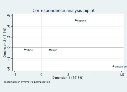
cabiplot , nocolumn yline(0) xline(0)
/* for ethnic */
cabiplot , nocolumn yline(0) xline(0)
 /* for ses */
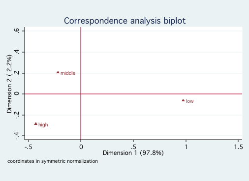
cabiplot , norow yline(0) xline(0)
/* for ses */
cabiplot , norow yline(0) xline(0)
Since both race and ses reflect socioeconomic factors, it is not surprising that
they fall primarily onto a single dimension. Looking at the first graph shows that White and Asian
are close to one another on Dimension 1, followed by Hispanic and further away African-American.
The second graph indicates that high and middle ses are close to one another with low ses much
further away. There is nothing in this analysis to contradict ones common sense interpretation of
these variables.Example 2
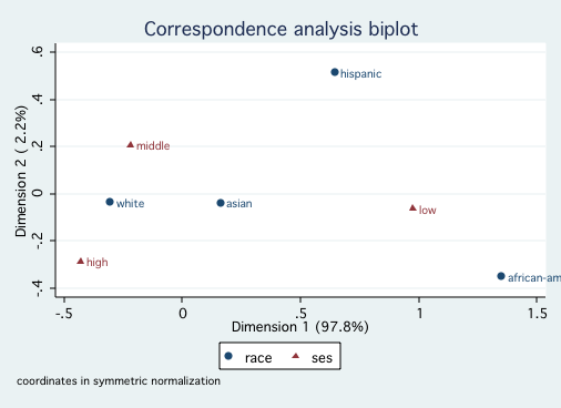
Next, we will try the same correspondence analysis separately by gender with numeric results suppressed.
quietly ca race ses if ~female cabiplot , yline(0) xline(0)Example 3quietly ca race ses if female cabiplot , yline(0) xline(0)
This is an example from the Stata manual using the matrix version of the command, camat. The data are from a 5x4 table giving the amount an individual smokes along with their job rank in a corporation.
                   level of smoking
  job rank    none   light  medium   heavy
  sen_mngr       4       2       3       2
  jun_mngr       4       3       7       4
  sen_empl      25      10      12       4
jun_employ      18      24      33      13
      secr      10       6       7       2
matrix F = ( 4,2,3,2 \ 4,3,7,4 \ 25,10,12,4 \ 18,24,33,13 \ 10,6,7,2 )
matrix colnames F = none light medium heavy
matrix rownames F = sen_mngr jun_mngr sen_empl jun_employ secr
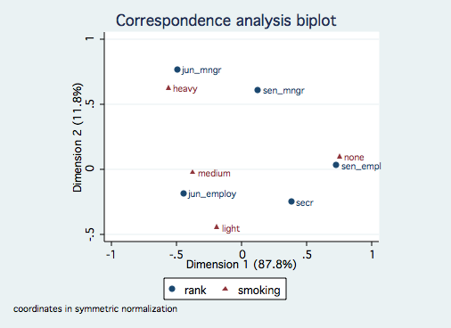
camat F, rowname(rank) colname(smoking) plot
Correspondence analysis Number of obs = 193
Pearson chi2(12) = 16.44
Prob > chi2 = 0.1718
Total inertia = 0.0852
5 active rows Number of dim. = 2
4 active columns Expl. inertia (%) = 99.51
| singular principal cumul
Dimensions | values inertia chi2 percent percent
-------------+-----------------------------------------------------------
dim 1 | .2734211 .0747591 14.43 87.76 87.76
dim 2 | .1000859 .0100172 1.93 11.76 99.51
dim 3 | .0203365 .0004136 0.08 0.49 100.00
-------------+-----------------------------------------------------------
total | .0851899 16.44 100
Statistics for row and column categories in symmetric normalization
| overall | dimension_1
Categories | mass quality inertia | coord sqcorr contrib
-------------+---------------------------+---------------------------
rank | |
sen mngr | 0.057 0.893 0.003 | 0.126 0.092 0.003
jun mngr | 0.093 0.991 0.012 | -0.495 0.526 0.084
sen empl | 0.264 1.000 0.038 | 0.728 0.999 0.512
jun employ | 0.456 1.000 0.026 | -0.446 0.942 0.331
secr | 0.130 0.999 0.006 | 0.385 0.865 0.070
-------------+---------------------------+---------------------------
smoking | |
none | 0.316 1.000 0.049 | 0.752 0.994 0.654
light | 0.233 0.984 0.007 | -0.190 0.327 0.031
medium | 0.321 0.983 0.013 | -0.375 0.982 0.166
heavy | 0.130 0.995 0.016 | -0.562 0.684 0.150
---------------------------------------------------------------------
| dimension_2
Categories | coord sqcorr contrib
-------------+---------------------------
rank |
sen mngr | 0.612 0.800 0.214
jun mngr | 0.769 0.465 0.551
sen empl | 0.034 0.001 0.003
jun employ | -0.183 0.058 0.152
secr | -0.249 0.133 0.081
-------------+---------------------------
smoking |
none | 0.096 0.006 0.029
light | -0.446 0.657 0.463
medium | -0.023 0.001 0.002
heavy | 0.625 0.310 0.506
-----------------------------------------
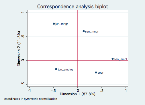
 cabiplot , nocolumn yline(0) xline(0)
 cabiplot , norow yline(0) xline(0)
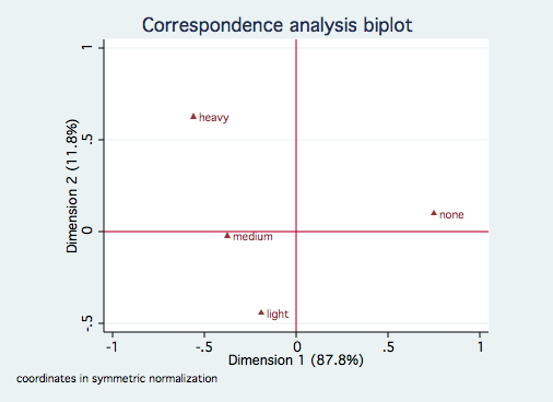
As with the previous example, there is only one significant dimension although dimension 2 does
account for nearly 12%. The smoking categories are reasonably ordered along dimension 1 from
"heavy" to "none." The job rank categories might be order by seniority, especially if
secretaries tend to be with the company longer than junior employees and junior managers.Multiple Correspondence Analysis Example
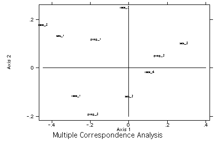
Using the user written command mca (findit mca) we will demonstrate a multiple correspondence analysis.
mca race ses prog, d(2)

------------------------------------------------------------------------------

                   MULTIPLE CORRESPONDENCE ANALYSIS

------------------------------------------------------------------------------


 Total Inertia :      0.053

 Principal Inertia Components :

      Inertia    Share    Cumul
Dim1    0.040    0.751    0.751
Dim2    0.012    0.225    0.976

 Coordinates :

           Mass  Inertia     Dim1     Dim2
race_1    0.040    0.004   -0.273   -0.120
race_2    0.018    0.001   -0.023    0.245
race_3    0.033    0.008   -0.447    0.173
race_4    0.242    0.003    0.109   -0.023
 ses_1    0.078    0.011   -0.357    0.128
 ses_2    0.158    0.003    0.002   -0.123
 ses_3    0.097    0.009    0.286    0.098
prog_1    0.075    0.003   -0.169    0.113
prog_2    0.175    0.005    0.161    0.046
prog_3    0.083    0.006   -0.185   -0.197

 Explained inertia of axes  :

          Dim1    Dim2
race_1  0.0749  0.0483
race_2  0.0002  0.0921
race_3  0.1665  0.0832
race_4  0.0714  0.0103
 ses_1  0.2505  0.1077
 ses_2  0.0000  0.2003
 ses_3  0.1984  0.0769
prog_1  0.0538  0.0800
prog_2  0.1130  0.0303
prog_3  0.0713  0.2709

 Contributions of principal axes :

          Dim1    Dim2
race_1  0.8161  0.1578
race_2  0.0067  0.7550
race_3  0.8554  0.1282
race_4  0.9557  0.0412
 ses_1  0.8833  0.1138
 ses_2  0.0002  0.9497
 ses_3  0.8873  0.1031
prog_1  0.6244  0.2782
prog_2  0.9081  0.0730
prog_3  0.4666  0.5316