
In this unit we will encounter the opposite situation from the zero-inflated models, we will look at data that have no zeros, the so called zero-truncated models. If one tries to use standard poisson or negative binomial analysis with these kinds of data the procedures try to fit the models by including probabilities for zero values. One should be able to produce more accurate models by using a probability model that does not include the zero values.
We will illustrate zero-truncated count models examining length of hospital stay (los) from the 1997 MedPar dataset. Length of stay does not and cannot have any zero values. Length of stay begins with a value of one and grows from there.
Stata 9 introduced two new commands ztp for zero-truncated poisson and ztnb for zero-truncated negative binomial. We will use both of these commands in this unit.
Note: The commands trpois0 and trnbin0 ado's and the medpar dataset were taken from a Stata Technical article (STB-47, January 1999) by Joseph Hilbe of Arizona State University can be used with Stata 8 and below.
Looking at the Data
The response variable in this example is length of hospital stay. With length of hospital stay, regardless of how little time is spent in the hospital, patients are credited as having at least one day.
use http://www.gseis.ucla.edu/courses/data/medpar, clear

describe

Contains data from medpar.dta
  obs:         1,495
 vars:            10                          30 Jun 1998 13:10
 size:        43,355 (98.6% of memory free)
-------------------------------------------------------------------------------
              storage  display     value
variable name   type   format      label      variable label
-------------------------------------------------------------------------------
provnum         str6   %9s                    Provider number
died            float  %9.0g
white           float  %9.0g
hmo             byte   %9.0g                  HMO/readmit'
los             int    %9.0g                  Length of Stay
age80           float  %9.0g
age             byte   %9.0g                  Age Group
type1           byte   %8.0g                  type==     1.0000
type2           byte   %8.0g                  type==     2.0000
type3           byte   %8.0g                  type==     3.0000
-------------------------------------------------------------------------------

summarize

    Variable |       Obs        Mean    Std. Dev.       Min        Max
-------------+--------------------------------------------------------
     provnum |         0
        died |      1495    .3431438    .4749179          0          1
       white |      1495    .9150502    .2789003          0          1
         hmo |      1495    .1598662    .3666046          0          1
         los |      1495    9.854181    8.832906          1        116
-------------+--------------------------------------------------------
       age80 |      1495    .2207358    .4148815          0          1
         age |      1495    5.235452    1.668898          1          9
       type1 |      1495    .7585284    .4281187          0          1
       type2 |      1495    .1772575    .3820143          0          1
       type3 |      1495     .064214    .2452159          0          1

tabstat los, stat(n mean sd var)

    variable |         N      mean        sd  variance
-------------+----------------------------------------
         los |      1495  9.854181  8.832906  78.02022
------------------------------------------------------

/* note: mean and variance are very different */

tabulate los

  Length of |
       Stay |      Freq.     Percent        Cum.
------------+-----------------------------------
          1 |        126        8.43        8.43
          2 |         71        4.75       13.18
          3 |         75        5.02       18.19
          4 |        104        6.96       25.15
          5 |        123        8.23       33.38
          6 |         97        6.49       39.87
          7 |        116        7.76       47.63
          8 |         92        6.15       53.78
          9 |         74        4.95       58.73
         10 |         89        5.95       64.68
         11 |         70        4.68       69.36
         12 |         70        4.68       74.05
         13 |         43        2.88       76.92
         14 |         49        3.28       80.20
         15 |         41        2.74       82.94
         16 |         43        2.88       85.82
         17 |         29        1.94       87.76
         18 |         23        1.54       89.30
         19 |         24        1.61       90.90
         20 |         19        1.27       92.17
         21 |         18        1.20       93.38
         22 |         15        1.00       94.38
         23 |         10        0.67       95.05
         24 |         11        0.74       95.79
         25 |          4        0.27       96.05
         26 |          7        0.47       96.52
         27 |          7        0.47       96.99
         28 |          5        0.33       97.32
         29 |          3        0.20       97.53
         30 |          1        0.07       97.59
         31 |          2        0.13       97.73
         32 |          6        0.40       98.13
         33 |          2        0.13       98.26
         34 |          5        0.33       98.60
         36 |          1        0.07       98.66
         42 |          1        0.07       98.73
         43 |          1        0.07       98.80
         44 |          2        0.13       98.93
         46 |          3        0.20       99.13
         48 |          1        0.07       99.20
         49 |          1        0.07       99.26
         50 |          1        0.07       99.33
         52 |          1        0.07       99.40
         57 |          1        0.07       99.46
         59 |          1        0.07       99.53
         60 |          1        0.07       99.60
         63 |          1        0.07       99.67
         65 |          1        0.07       99.73
         70 |          1        0.07       99.80
         74 |          1        0.07       99.87
         91 |          1        0.07       99.93
        116 |          1        0.07      100.00
------------+-----------------------------------
      Total |      1,495      100.00

nbvargr los, n(15)

Obtaining Parameter Estimates

(36 observations deleted)
here

  Negative Binomial Probabilities
  with mean = 9.854181 & overdispersion = .4902339

     +------------------------------+
     |  k       nbprob        nbcum |
     |------------------------------|
  1. |  0   0.02741744   0.02741744 |
  2. |  1   0.04633566   0.07375310 |
  3. |  2   0.05834830   0.13210140 |
  4. |  3   0.06509732   0.19719872 |
  5. |  4   0.06795350   0.26515222 |
     |------------------------------|
  6. |  5   0.06800788   0.33316010 |
  7. |  6   0.06610931   0.39926943 |
  8. |  7   0.06290771   0.46217713 |
  9. |  8   0.05889338   0.52107054 |
 10. |  9   0.05443054   0.57550102 |
     |------------------------------|
 11. | 10   0.04978486   0.62528592 |
 12. | 11   0.04514578   0.67043167 |
 13. | 12   0.04064433   0.71107602 |
 14. | 13   0.03636726   0.74744326 |
 15. | 14   0.03236813   0.77981138 |
     |------------------------------|
 16. | 15   0.02867597   0.80848736 |
     +------------------------------+
k was int now float

 Poisson Probabilities for lambda = 9.854181

     +------------------------------+
     |  k        pprob         pcum |
     |------------------------------|
  1. |  0   0.00005253   0.00005253 |
  2. |  1   0.00051761   0.00057014 |
  3. |  2   0.00255032   0.00312046 |
  4. |  3   0.00837710   0.01149756 |
  5. |  4   0.02063738   0.03213494 |
     |------------------------------|
  6. |  5   0.04067289   0.07280783 |
  7. |  6   0.06679966   0.13960749 |
  8. |  7   0.09403657   0.23364405 |
  9. |  8   0.11583167   0.34947574 |
 10. |  9   0.12682514   0.47630087 |
     |------------------------------|
 11. | 10   0.12497579   0.60127664 |
 12. | 11   0.11195764   0.71323431 |
 13. | 12   0.09193757   0.80517185 |
 14. | 13   0.06968996   0.87486184 |
 15. | 14   0.04905268   0.92391449 |
     |------------------------------|
 16. | 15   0.03222493   0.95613945 |
     +------------------------------+
(1 observation deleted)
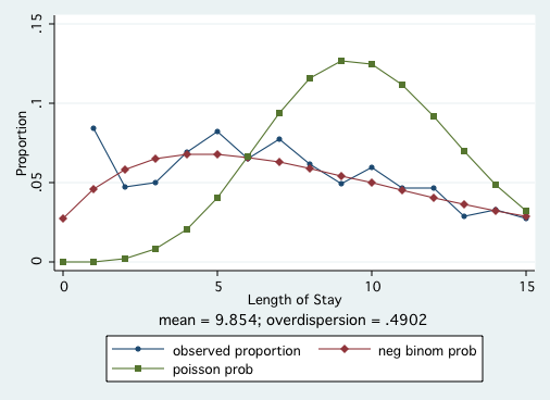
Tricking StataIts clear from the nbvargr that neither the poisson and negative binomial distributions fit the observed data very well. Also, the negative binomial distribution expects that there will be some (approximately 40) zero values.
We will run standard poisson and negative binomial regressions and then we will trick Stata by subtracting one from the value of length of stay and rerunning these models.
poisson los died hmo type2 type3, nolog cluster(provnum)
Poisson regression Number of obs = 1495
Wald chi2(4) = 30.71
Log pseudolikelihood = -6846.9485 Prob > chi2 = 0.0000
(Std. Err. adjusted for 54 clusters in provnum)
------------------------------------------------------------------------------
| Robust
los | Coef. Std. Err. z P>|z| [95% Conf. Interval]
-------------+----------------------------------------------------------------
died | -.2483158 .0633446 -3.92 0.000 -.3724689 -.1241627
hmo | -.0753708 .0502589 -1.50 0.134 -.1738764 .0231348
type2 | .2498558 .0646699 3.86 0.000 .1231051 .3766066
type3 | .7501452 .2184939 3.43 0.001 .3219049 1.178385
_cons | 2.264575 .0335312 67.54 0.000 2.198855 2.330295
------------------------------------------------------------------------------
/* compute aic */
display (-2*-6846.948518+2*4)/1495
9.1651485
nbreg los died hmo type2 type3, nolog cluster(provnum)
Negative binomial regression Number of obs = 1495
Dispersion = mean Wald chi2(4) = 36.13
Log pseudolikelihood = -4782.5989 Prob > chi2 = 0.0000
(Std. Err. adjusted for 54 clusters in provnum)
------------------------------------------------------------------------------
| Robust
los | Coef. Std. Err. z P>|z| [95% Conf. Interval]
-------------+----------------------------------------------------------------
died | -.236979 .0573431 -4.13 0.000 -.3493694 -.1245886
hmo | -.0705928 .049645 -1.42 0.155 -.1678953 .0267097
type2 | .2532097 .0634972 3.99 0.000 .1287575 .3776619
type3 | .7365274 .2115372 3.48 0.000 .3219221 1.151133
_cons | 2.260834 .0327839 68.96 0.000 2.196578 2.325089
-------------+----------------------------------------------------------------
/lnalpha | -.8318959 .0634521 -.9562597 -.707532
-------------+----------------------------------------------------------------
alpha | .4352234 .0276158 .3843277 .4928591
------------------------------------------------------------------------------
/* compute aic */
display (-2*-4782.5989+2*4)/1495
6.4034768
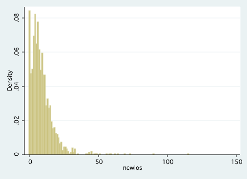
/* create new variable with zero */
generate newlos = los - 1
histogram newlos, discrete
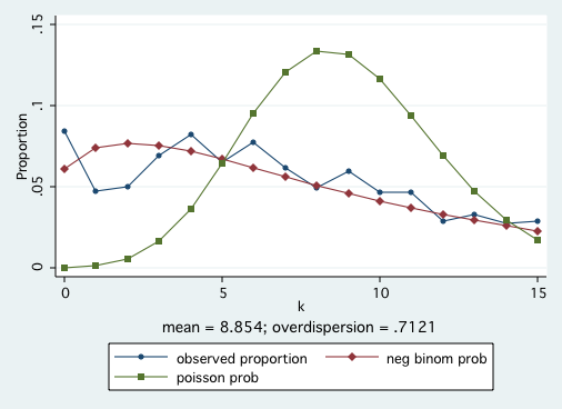
 nbvargr newlos, n(15)
Obtaining Parameter Estimates
(36 observations deleted)
here
Negative Binomial Probabilities
with mean = 8.854181 & overdispersion = .7120889
+------------------------------+
| k nbprob nbcum |
|------------------------------|
1. | 0 0.06126391 0.06126391 |
2. | 1 0.07425659 0.13552050 |
3. | 2 0.07704805 0.21256854 |
4. | 3 0.07546319 0.28803173 |
5. | 4 0.07171640 0.35974813 |
|------------------------------|
6. | 5 0.06690429 0.42665243 |
7. | 6 0.06163682 0.48828924 |
8. | 7 0.05627193 0.54456115 |
9. | 8 0.05102334 0.59558451 |
10. | 9 0.04601700 0.64160150 |
|------------------------------|
11. | 10 0.04132344 0.68292499 |
12. | 11 0.03697751 0.71990246 |
13. | 12 0.03299088 0.75289333 |
14. | 13 0.02936026 0.78225362 |
15. | 14 0.02607288 0.80832648 |
|------------------------------|
16. | 15 0.02311026 0.83143675 |
+------------------------------+
Poisson Probabilities for lambda = 8.854181
+------------------------------+
| k pprob pcum |
|------------------------------|
1. | 0 0.00014278 0.00014278 |
2. | 1 0.00126423 0.00140701 |
3. | 2 0.00559686 0.00700388 |
4. | 3 0.01651855 0.02352243 |
5. | 4 0.03656456 0.06008700 |
|------------------------------|
6. | 5 0.06474985 0.12483685 |
7. | 6 0.09555116 0.22038800 |
8. | 7 0.12086103 0.34124902 |
9. | 8 0.13376568 0.47501472 |
10. | 9 0.13159840 0.60661310 |
|------------------------------|
11. | 10 0.11651960 0.72313273 |
12. | 11 0.09378960 0.81692231 |
13. | 12 0.06920251 0.88612479 |
14. | 13 0.04713320 0.93325800 |
15. | 14 0.02980899 0.96306700 |
|------------------------------|
16. | 15 0.01759561 0.98066264 |
+------------------------------+
(0 observations deleted)
nbvargr newlos, n(15)
Obtaining Parameter Estimates
(36 observations deleted)
here
Negative Binomial Probabilities
with mean = 8.854181 & overdispersion = .7120889
+------------------------------+
| k nbprob nbcum |
|------------------------------|
1. | 0 0.06126391 0.06126391 |
2. | 1 0.07425659 0.13552050 |
3. | 2 0.07704805 0.21256854 |
4. | 3 0.07546319 0.28803173 |
5. | 4 0.07171640 0.35974813 |
|------------------------------|
6. | 5 0.06690429 0.42665243 |
7. | 6 0.06163682 0.48828924 |
8. | 7 0.05627193 0.54456115 |
9. | 8 0.05102334 0.59558451 |
10. | 9 0.04601700 0.64160150 |
|------------------------------|
11. | 10 0.04132344 0.68292499 |
12. | 11 0.03697751 0.71990246 |
13. | 12 0.03299088 0.75289333 |
14. | 13 0.02936026 0.78225362 |
15. | 14 0.02607288 0.80832648 |
|------------------------------|
16. | 15 0.02311026 0.83143675 |
+------------------------------+
Poisson Probabilities for lambda = 8.854181
+------------------------------+
| k pprob pcum |
|------------------------------|
1. | 0 0.00014278 0.00014278 |
2. | 1 0.00126423 0.00140701 |
3. | 2 0.00559686 0.00700388 |
4. | 3 0.01651855 0.02352243 |
5. | 4 0.03656456 0.06008700 |
|------------------------------|
6. | 5 0.06474985 0.12483685 |
7. | 6 0.09555116 0.22038800 |
8. | 7 0.12086103 0.34124902 |
9. | 8 0.13376568 0.47501472 |
10. | 9 0.13159840 0.60661310 |
|------------------------------|
11. | 10 0.11651960 0.72313273 |
12. | 11 0.09378960 0.81692231 |
13. | 12 0.06920251 0.88612479 |
14. | 13 0.04713320 0.93325800 |
15. | 14 0.02980899 0.96306700 |
|------------------------------|
16. | 15 0.01759561 0.98066264 |
+------------------------------+
(0 observations deleted)
 poisson newlos died hmo type2 type3, nolog cluster(provnum)
Poisson regression Number of obs = 1495
Wald chi2(4) = 31.42
Log pseudolikelihood = -7229.6375 Prob > chi2 = 0.0000
(Std. Err. adjusted for 54 clusters in provnum)
------------------------------------------------------------------------------
| Robust
newlos | Coef. Std. Err. z P>|z| [95% Conf. Interval]
-------------+----------------------------------------------------------------
died | -.277442 .0703259 -3.95 0.000 -.4152782 -.1396057
hmo | -.0849026 .056734 -1.50 0.135 -.1960993 .0262941
type2 | .2778412 .071253 3.90 0.000 .1381879 .4174945
type3 | .8166476 .2318683 3.52 0.000 .3621941 1.271101
_cons | 2.153754 .0372609 57.80 0.000 2.080724 2.226784
------------------------------------------------------------------------------
/* compute aic */
display (-2*-7229.6375+2*4)/1495
9.677107
nbreg newlos died hmo type2 type3, nolog cluster(provnum)
Negative binomial regression Number of obs = 1495
Dispersion = mean Wald chi2(4) = 37.00
Log pseudolikelihood = -4742.6087 Prob > chi2 = 0.0000
(Std. Err. adjusted for 54 clusters in provnum)
------------------------------------------------------------------------------
| Robust
newlos | Coef. Std. Err. z P>|z| [95% Conf. Interval]
-------------+----------------------------------------------------------------
died | -.2650532 .0644419 -4.11 0.000 -.3913571 -.1387494
hmo | -.0793184 .0563 -1.41 0.159 -.1896643 .0310275
type2 | .2826808 .069884 4.05 0.000 .1457107 .4196509
type3 | .8011306 .224282 3.57 0.000 .361546 1.240715
_cons | 2.149526 .0365384 58.83 0.000 2.077912 2.22114
-------------+----------------------------------------------------------------
/lnalpha | -.448078 .0559217 -.5576824 -.3384736
-------------+----------------------------------------------------------------
alpha | .6388549 .0357258 .5725344 .7128576
------------------------------------------------------------------------------
/* compute aic */
display (-2*-4742.6087+2*4)/1495
6.3499782
/* Summary Table
variable model log likelihood aic
los poisson -6846.9485 9.1651485
los nbreg -4782.5989 6.4034768
newlos poisson -7229.6375 9.677107
newlos nbreg -4742.6087 6.3499782 */
poisson newlos died hmo type2 type3, nolog cluster(provnum)
Poisson regression Number of obs = 1495
Wald chi2(4) = 31.42
Log pseudolikelihood = -7229.6375 Prob > chi2 = 0.0000
(Std. Err. adjusted for 54 clusters in provnum)
------------------------------------------------------------------------------
| Robust
newlos | Coef. Std. Err. z P>|z| [95% Conf. Interval]
-------------+----------------------------------------------------------------
died | -.277442 .0703259 -3.95 0.000 -.4152782 -.1396057
hmo | -.0849026 .056734 -1.50 0.135 -.1960993 .0262941
type2 | .2778412 .071253 3.90 0.000 .1381879 .4174945
type3 | .8166476 .2318683 3.52 0.000 .3621941 1.271101
_cons | 2.153754 .0372609 57.80 0.000 2.080724 2.226784
------------------------------------------------------------------------------
/* compute aic */
display (-2*-7229.6375+2*4)/1495
9.677107
nbreg newlos died hmo type2 type3, nolog cluster(provnum)
Negative binomial regression Number of obs = 1495
Dispersion = mean Wald chi2(4) = 37.00
Log pseudolikelihood = -4742.6087 Prob > chi2 = 0.0000
(Std. Err. adjusted for 54 clusters in provnum)
------------------------------------------------------------------------------
| Robust
newlos | Coef. Std. Err. z P>|z| [95% Conf. Interval]
-------------+----------------------------------------------------------------
died | -.2650532 .0644419 -4.11 0.000 -.3913571 -.1387494
hmo | -.0793184 .0563 -1.41 0.159 -.1896643 .0310275
type2 | .2826808 .069884 4.05 0.000 .1457107 .4196509
type3 | .8011306 .224282 3.57 0.000 .361546 1.240715
_cons | 2.149526 .0365384 58.83 0.000 2.077912 2.22114
-------------+----------------------------------------------------------------
/lnalpha | -.448078 .0559217 -.5576824 -.3384736
-------------+----------------------------------------------------------------
alpha | .6388549 .0357258 .5725344 .7128576
------------------------------------------------------------------------------
/* compute aic */
display (-2*-4742.6087+2*4)/1495
6.3499782
/* Summary Table
variable model log likelihood aic
los poisson -6846.9485 9.1651485
los nbreg -4782.5989 6.4034768
newlos poisson -7229.6375 9.677107
newlos nbreg -4742.6087 6.3499782 */
The negative binomial regression with the trick is only slightly
better and the poisson regression with the trick is actually worse.Zero-truncated Poisson
We will begin the zero-truncated models with a zero-truncated poisson regression even though it is unlikely that a poisson distribution will be appropriate for these data since the mean and variance of los are nowhere near equal.
ztp los died hmo type2 type3, nolog cluster(provnum)

Zero-truncated Poisson regression                 Number of obs   =       1495
                                                  Wald chi2(4)    =      30.68
Log pseudolikelihood = -6846.6528                 Prob > chi2     =     0.0000

                               (Std. Err. adjusted for 54 clusters in provnum)
------------------------------------------------------------------------------
             |               Robust
         los |      Coef.   Std. Err.      z    P>|z|     [95% Conf. Interval]
-------------+----------------------------------------------------------------
        died |   -.248681   .0634856    -3.92   0.000    -.3731105   -.1242514
         hmo |  -.0755112   .0503728    -1.50   0.134    -.1742401    .0232177
       type2 |   .2500681   .0647042     3.86   0.000     .1232501     .376886
       type3 |   .7503999   .2185408     3.43   0.001     .3220678    1.178732
       _cons |   2.264474   .0335532    67.49   0.000     2.198711    2.330237
------------------------------------------------------------------------------

/* compute aic */
display (-2*-6846.6528+2*4)/1495

9.1647529

ztp, irr

Zero-truncated Poisson regression                 Number of obs   =       1495
                                                  Wald chi2(4)    =      30.68
Log pseudolikelihood = -6846.6528                 Prob > chi2     =     0.0000

                               (Std. Err. adjusted for 54 clusters in provnum)
------------------------------------------------------------------------------
             |               Robust
         los |        IRR   Std. Err.      z    P>|z|     [95% Conf. Interval]
-------------+----------------------------------------------------------------
        died |   .7798287   .0495079    -3.92   0.000     .6885891    .8831577
         hmo |   .9272693   .0467091    -1.50   0.134     .8400952    1.023489
       type2 |   1.284113   .0830875     3.86   0.000     1.131167    1.457738
       type3 |   2.117847    .462836     3.43   0.001     1.379978    3.250251
------------------------------------------------------------------------------
Zero-truncated Negative Binomial
ztnb los died hmo type2 type3, nolog cluster(provnum)

Zero-truncated negative binomial regression       Number of obs   =       1495
Dispersion     = mean                             Wald chi2(4)    =      36.01
Log likelihood = -4737.535                        Prob > chi2     =     0.0000

                               (Std. Err. adjusted for 54 clusters in provnum)
------------------------------------------------------------------------------
             |               Robust
         los |      Coef.   Std. Err.      z    P>|z|     [95% Conf. Interval]
-------------+----------------------------------------------------------------
        died |  -.2521884    .061533    -4.10   0.000    -.3727908   -.1315859
         hmo |  -.0754173   .0533132    -1.41   0.157    -.1799091    .0290746
       type2 |   .2685095   .0666474     4.03   0.000      .137883    .3991359
       type3 |   .7668101   .2183505     3.51   0.000      .338851    1.194769
       _cons |   2.224028    .034727    64.04   0.000     2.155964    2.292091
-------------+----------------------------------------------------------------
    /lnalpha |   -.630108   .0764019                      -.779853    -.480363
-------------+----------------------------------------------------------------
       alpha |   .5325343   .0406866                      .4584734    .6185588
------------------------------------------------------------------------------

/* compute aic */
display (-2*-4782.5989+2*4)/1495

6.4034768

ztnb, irr

Zero-truncated negative binomial regression       Number of obs   =       1495
Dispersion     = mean                             Wald chi2(4)    =      36.01
Log likelihood = -4737.535                        Prob > chi2     =     0.0000

                               (Std. Err. adjusted for 54 clusters in provnum)
------------------------------------------------------------------------------
             |               Robust
         los |        IRR   Std. Err.      z    P>|z|     [95% Conf. Interval]
-------------+----------------------------------------------------------------
        died |   .7770984   .0478172    -4.10   0.000     .6888093    .8767039
         hmo |   .9273564   .0494403    -1.41   0.157     .8353461    1.029501
       type2 |   1.308013   .0871756     4.03   0.000     1.147841    1.490536
       type3 |   2.152888   .4700841     3.51   0.000     1.403334    3.302795
-------------+----------------------------------------------------------------
    /lnalpha |   -.630108   .0764019                      -.779853    -.480363
-------------+----------------------------------------------------------------
       alpha |   .5325343   .0406866                      .4584734    .6185588
------------------------------------------------------------------------------

predict plos

tablist los plos, sort(v) clean

   los       plos   Freq
      1   6.662014     18
      1   7.183877     70
      1   8.572936      2
      1   8.714004      2
      1   9.244488     13
      1   9.396606      8
      1   12.09191      7
      1   15.46608      4
      1   19.90235      2
      2   6.662014      7
      2   7.183877     22
      2   8.572936      3
      2   9.244488     22
      2   9.396606      5
      2   12.09191      6
      2   15.46608      5
      2   19.90235      1
      3   6.662014      3
      3   7.183877     17
      3   8.572936      9
      3   8.714004      2
      3   9.244488     33
      3   9.396606      5
      3   11.21351      1
      3   12.09191      2
      3   15.46608      3
      4   6.662014      5
      4   7.183877     15
      4   8.572936     11
      4   8.714004      1
      4   9.244488     50
      4   9.396606      9
      4   11.21351      1
      4   12.09191      8
      4   15.46608      2
      4   19.90235      2
      5   6.662014      2
      5   7.183877     19
      5   8.572936     16
      5   9.244488     61
      5   9.396606      5
      5   11.21351      3
      5   12.09191      9
      5   14.34257      1
      5   15.46608      5
      5   18.45657      1
      5   19.90235      1
      6   6.662014      3
      6   7.183877     10
      6   8.572936     11
      6   9.244488     50
      6   9.396606      6
      6   11.21351      2
      6   12.09191     11
      6   15.46608      1
      6   19.90235      3
      7   6.662014      3
      7   7.183877     20
      7   8.572936     16
      7   8.714004      1
      7   9.244488     54
      7   9.396606     10
      7   11.21351      2
      7   12.09191      8
      7   15.46608      1
      7   19.90235      1
      8   6.662014      3
      8   7.183877     18
      8   8.572936      8
      8   8.714004      1
      8   9.244488     49
      8   9.396606      4
      8   12.09191      7
      8   15.46608      1
      8   19.90235      1
      9   6.662014      3
      9   7.183877      5
      9   8.572936     15
      9   9.244488     34
      9   9.396606      7
      9   12.09191      6
      9   15.46608      1
      9   19.90235      3
     10   6.662014      3
     10   7.183877     18
     10   8.572936      2
     10   9.244488     53
     10   9.396606      2
     10   12.09191      7
     10   15.46608      1
     10   19.90235      3
     11   6.662014      3
     11   7.183877     10
     11   8.572936      9
     11   9.244488     32
     11   9.396606      1
     11   11.21351      1
     11   12.09191      8
     11   15.46608      2
     11   19.90235      4
     12   6.662014      2
     12   7.183877     10
     12   8.572936      6
     12   9.244488     35
     12   9.396606      3
     12   11.21351      2
     12   12.09191     10
     12   19.90235      2
     13   6.662014      3
     13   7.183877      6
     13   8.572936      5
     13   9.244488     19
     13   9.396606      2
     13   11.21351      1
     13   12.09191      6
     13   15.46608      1
     14   6.662014      6
     14   7.183877      9
     14   8.572936      3
     14   9.244488     19
     14   9.396606      3
     14   11.21351      2
     14   12.09191      3
     14   15.46608      1
     14   19.90235      3
     15   6.662014      1
     15   7.183877      6
     15   8.572936      2
     15   9.244488     18
     15   9.396606      3
     15   12.09191      8
     15   19.90235      3
     16   7.183877      8
     16   8.572936      2
     16   9.244488     15
     16   9.396606      1
     16   11.21351      2
     16   12.09191     12
     16   15.46608      2
     16   19.90235      1
     17   6.662014      1
     17   7.183877      6
     17   8.572936      3
     17   9.244488     11
     17   9.396606      4
     17   15.46608      2
     17   18.45657      1
     17   19.90235      1
     18   6.662014      1
     18   7.183877      3
     18   8.572936      3
     18   8.714004      1
     18   9.244488     13
     18   12.09191      1
     18   19.90235      1
     19   6.662014      1
     19   7.183877      2
     19   8.572936      3
     19   8.714004      2
     19   9.244488      8
     19   12.09191      4
     19   15.46608      4
     20   6.662014      1
     20   7.183877      4
     20   9.244488      9
     20   9.396606      2
     20   12.09191      3
     21   7.183877      3
     21   8.572936      1
     21   9.244488      8
     21   9.396606      2
     21   11.21351      1
     21   12.09191      3
     22   7.183877      2
     22   8.572936      1
     22   8.714004      1
     22   9.244488      4
     22   9.396606      1
     22   12.09191      2
     22   15.46608      3
     22   19.90235      1
     23   7.183877      1
     23   8.572936      2
     23   9.244488      6
     23   9.396606      1
     24   7.183877      3
     24   9.244488      5
     24   9.396606      2
     24   19.90235      1
     25   7.183877      2
     25   9.244488      2
     26   7.183877      2
     26   9.244488      2
     26   12.09191      2
     26   19.90235      1
     27   7.183877      1
     27   9.244488      1
     27   9.396606      1
     27   11.21351      1
     27   12.09191      1
     27   19.90235      2
     28   9.244488      1
     28   9.396606      1
     28   12.09191      1
     28   15.46608      2
     29   8.572936      1
     29   9.244488      1
     29   19.90235      1
     30   9.396606      1
     31   8.572936      1
     31   9.244488      1
     32   7.183877      1
     32   9.244488      2
     32   9.396606      1
     32   12.09191      1
     32   19.90235      1
     33   9.244488      1
     33   9.396606      1
     34   9.244488      1
     34   9.396606      2
     34   11.21351      1
     34   12.09191      1
     36   6.662014      1
     42   19.90235      1
     43   12.09191      1
     44   12.09191      2
     46   9.244488      1
     46   19.90235      2
     48   19.90235      1
     49   15.46608      1
     50   7.183877      1
     52   19.90235      1
     57   19.90235      1
     59   19.90235      1
     60   9.244488      1
     63   12.09191      1
     65   19.90235      1
     70   15.46608      1
     74   19.90235      1
     91   15.46608      1
    116   19.90235      1

tab plos

  predicted |
  number of |
     events |      Freq.     Percent        Cum.
------------+-----------------------------------
   6.662014 |         70        4.68        4.68
   7.183877 |        294       19.67       24.35
   8.572936 |        135        9.03       33.38
   8.714004 |         11        0.74       34.11
   9.244488 |        635       42.47       76.59
   9.396606 |         93        6.22       82.81
   11.21351 |         20        1.34       84.15
   12.09191 |        141        9.43       93.58
   14.34257 |          1        0.07       93.65
   15.46608 |         44        2.94       96.59
   18.45657 |          2        0.13       96.72
   19.90235 |         49        3.28      100.00
------------+-----------------------------------
      Total |      1,495      100.00

univar los plos

                                        -------------- Quantiles --------------
Variable       n     Mean     S.D.      Min      .25      Mdn      .75      Max
-------------------------------------------------------------------------------
     los    1495     9.85     8.83     1.00     4.00     8.00    13.00   116.00
    plos    1495     9.51     2.63     6.66     8.57     9.24     9.24    19.90
-------------------------------------------------------------------------------

corr los plos
(obs=1495)

             |      los     plos
-------------+------------------
         los |   1.0000
        plos |   0.3060   1.0000


/* Summary Table
      variable  model     log likelihood     aic
      los       poisson     -6846.9485       9.1651485
      los       nbreg       -4782.5989       6.4034768
      newlos    poisson     -7229.6375       9.677107
      newlos    nbreg       -4742.6087       6.3499782
      los       zpt         -6846.6528       9.1647529
      los       ztnb        -4737.535        6.3431906 */
The zero-truncated models provided only a slight improvement over the negative binomial with
the subtraction trick and also slightly better for than the standrad poisson regression.In the final analysis, the predicted counts 't seem to match the observed counts only moderately well. This may be due, in part, to the fact that there are only eight different covariate patterns among the predictors, one of which, was not significant.