
Analyzing data that contain censored values or are truncated is common in many research disciplines. According to Hosmer and Lemeshow (1999), a censored value is one whose value is incomplete due to random factors for each subject. A truncated observation, on the other hand, is one which is incomplete due to a selection process in the design of the study. Thus, truncation changes the sample size while censoring does not.
We will begin by looking at analyzing data with censored values.
Regression with Censored Data
Regression models with censored data are sometimes called tobit models, named for the estimation that was originally developed by J. Tobin (1958).
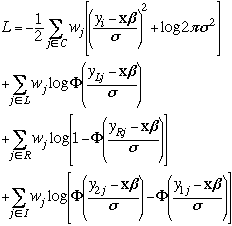
The log likelihood for the general model with censored data looks like
Let's start off with an example from Long (1997), the data are available from www.indiana.edu/~jsl650 (the data file is called job1tob.dta). This example looks at the prestige of a scientist's first job. Job prestige values were not available for departments without graduate programs or for graduate programs rated below 1.0. These cases were coded as ones. In this example, some of the ones represent 'true' ones, while the others are censored values that are less than one but whose 'true' values are unknown.
First we will looks at the OLS analysis with the censored data. With this approach all of the values scored as one are treated as if they were 'true' ones.
use http://www.gseis.ucla.edu/courses/data/job1tob

summarize jobcen0 jobcen1

    Variable |     Obs        Mean   Std. Dev.       Min        Max
-------------+-----------------------------------------------------
     jobcen0 |     408    1.990784    1.31612          0        4.8
     jobcen1 |     408    2.233431   .9736029          1        4.8

regress jobcen1 fem phd ment fel art cit

      Source |       SS       df       MS              Number of obs =     408
-------------+------------------------------           F(  6,   401) =   17.78
       Model |  81.0584763     6  13.5097461           Prob > F      =  0.0000
    Residual |  304.737915   401  .759944926           R-squared     =  0.2101
-------------+------------------------------           Adj R-squared =  0.1983
       Total |  385.796392   407  .947902683           Root MSE      =  .87175

------------------------------------------------------------------------------
     jobcen1 |      Coef.   Std. Err.      t    P>|t|     [95% Conf. Interval]
-------------+----------------------------------------------------------------
         fem |  -.1391939   .0902344    -1.54   0.124    -.3165856    .0381977
         phd |   .2726826   .0493183     5.53   0.000     .1757278    .3696375
        ment |   .0011867   .0007012     1.69   0.091    -.0001917    .0025651
         fel |   .2341384   .0948206     2.47   0.014     .0477308    .4205461
         art |   .0228011   .0288843     0.79   0.430    -.0339824    .0795846
         cit |   .0044788   .0019687     2.28   0.023     .0006087     .008349
       _cons |   1.067184   .1661357     6.42   0.000     .7405785     1.39379
------------------------------------------------------------------------------

listcoef

regress (N=408): Unstandardized and Standardized Estimates

 Observed SD: .97360294
 SD of Error: .8717482

---------------------------------------------------------------------------
 jobcen1 |      b         t     P>|t|    bStdX    bStdY   bStdXY      SDofX
---------+-----------------------------------------------------------------
     fem |  -0.13919   -1.543   0.124  -0.0680  -0.1430  -0.0698     0.4883
     phd |   0.27268    5.529   0.000   0.2601   0.2801   0.2671     0.9538
    ment |   0.00119    1.692   0.091   0.0778   0.0012   0.0799    65.5299
     fel |   0.23414    2.469   0.014   0.1139   0.2405   0.1170     0.4866
     art |   0.02280    0.789   0.430   0.0514   0.0234   0.0528     2.2561
     cit |   0.00448    2.275   0.023   0.1481   0.0046   0.1521    33.0599
---------------------------------------------------------------------------
Next, we will perform an OLS regression after dropping out all of the cases that had been
censored to one. In this analysis, all of the ones are 'true' ones, the other values
are deleted. We have truncated the sample by dropping all prestige ratings less than
one.
regress jobcen0 fem phd ment fel art cit if jobcen0 ~= 0

      Source |       SS       df       MS              Number of obs =     309
-------------+------------------------------           F(  6,   302) =   12.69
       Model |  37.6365095     6  6.27275158           Prob > F      =  0.0000
    Residual |  149.290989   302  .494341024           R-squared     =  0.2013
-------------+------------------------------           Adj R-squared =  0.1855
       Total |  186.927499   308  .606907463           Root MSE      =  .70309

------------------------------------------------------------------------------
     jobcen0 |      Coef.   Std. Err.      t    P>|t|     [95% Conf. Interval]
-------------+----------------------------------------------------------------
         fem |   .1014513   .0854827     1.19   0.236    -.0667658    .2696685
         phd |   .2973797   .0467477     6.36   0.000     .2053873    .3893722
        ment |   .0007784   .0006113     1.27   0.204    -.0004247    .0019814
         fel |   .1405303   .0897917     1.57   0.119    -.0361662    .3172269
         art |   .0058978   .0248279     0.24   0.812    -.0429598    .0547554
         cit |   .0021032   .0016553     1.27   0.205    -.0011542    .0053607
       _cons |   1.412782   .1621386     8.71   0.000     1.093718    1.731846
------------------------------------------------------------------------------

listcoef

regress (N=309): Unstandardized and Standardized Estimates

 Observed SD: .77904266
 SD of Error: .70309389

---------------------------------------------------------------------------
 jobcen0 |      b         t     P>|t|    bStdX    bStdY   bStdXY      SDofX
---------+-----------------------------------------------------------------
     fem |   0.10145    1.187   0.236   0.0481   0.1302   0.0618     0.4744
     phd |   0.29738    6.361   0.000   0.2758   0.3817   0.3540     0.9274
    ment |   0.00078    1.273   0.204   0.0541   0.0010   0.0695    69.5468
     fel |   0.14053    1.565   0.119   0.0662   0.1804   0.0850     0.4710
     art |   0.00590    0.238   0.812   0.0142   0.0076   0.0182     2.4000
     cit |   0.00210    1.271   0.205   0.0760   0.0027   0.0976    36.1466
---------------------------------------------------------------------------
Finally, we will estimate a model using the tobit method. It includes those cases that were censored
to a value of one. We will declare the data to be left censored at 1.0. Using information in the
sample, the tobit procedure computes the probability that a value of one is censored and uses
the probability to aid in the estimation of the coefficients.
tobit jobcen1 fem phd ment fel art cit, ll(1)

Tobit estimates                                   Number of obs   =        408
                                                  LR chi2(6)      =      89.20
                                                  Prob > chi2     =     0.0000
Log likelihood = -560.25209                       Pseudo R2       =     0.0737

------------------------------------------------------------------------------
     jobcen1 |      Coef.   Std. Err.      t    P>|t|     [95% Conf. Interval]
-------------+----------------------------------------------------------------
         fem |  -.2368486   .1165795    -2.03   0.043    -.4660302   -.0076669
         phd |   .3225846   .0639198     5.05   0.000     .1969258    .4482435
        ment |   .0013436   .0008875     1.51   0.131    -.0004011    .0030884
         fel |   .3252657   .1224516     2.66   0.008     .0845403    .5659911
         art |   .0339053      .0365     0.93   0.353    -.0378493      .10566
         cit |     .00509   .0024751     2.06   0.040     .0002243    .0099557
       _cons |   .6854061    .218261     3.14   0.002     .2563307    1.114482
-------------+----------------------------------------------------------------
         _se |   1.087237    .046533           (Ancillary parameter)
------------------------------------------------------------------------------

  Obs. summary:         99  left-censored observations at jobcen1<=1
                       309     uncensored observations

listcoef

tobit (N=408): Unstandardized and Standardized Estimates

 Observed SD: .97360294
   Latent SD: 1.21966
 SD of Error: 1.087237

---------------------------------------------------------------------------
 jobcen1 |      b         t     P>|t|    bStdX    bStdY   bStdXY      SDofX
---------+-----------------------------------------------------------------
     fem |  -0.23685   -2.032   0.043  -0.1156  -0.1942  -0.0948     0.4883
     phd |   0.32258    5.047   0.000   0.3077   0.2645   0.2523     0.9538
    ment |   0.00134    1.514   0.131   0.0880   0.0011   0.0722    65.5299
     fel |   0.32527    2.656   0.008   0.1583   0.2667   0.1298     0.4866
     art |   0.03391    0.929   0.353   0.0765   0.0278   0.0627     2.2561
     cit |   0.00509    2.057   0.040   0.1683   0.0042   0.1380    33.0599
---------------------------------------------------------------------------
In the next example we have a variable called acadindx which is a weighted combination
of standardized test scores and academic grades. The maximum possible score on
acadindx is 200 but it is clear that the 26 students who scored 200 are not exactly
equal in their academic abilities. In other words, there is variability in
academic ability that is not being accounted for when students score 200 on
acadindx. Acadindx is right censored and in this sample, we do not know which students have
'true' scores of 200 and which ones have censored scores.We will begin by looking at a description of the data, some descriptive statistics, and correlations among the variables.
use http://www.gseis.ucla.edu/courses/data/acadindx2
(max possible on acadindx is 200)

describe

Contains data from acadindx.dta
  obs:           200                          max possible on acadindx is 200
 vars:             5                          19 Jan 2001 20:14
 size:         4,800 (99.7% of memory free)
-------------------------------------------------------------------------------
   1. id        float  %9.0g
   2. female    float  %9.0g       fl
   3. reading   float  %9.0g
   4. writing   float  %9.0g
   5. acadindx  float  %9.0g                  academic index
-------------------------------------------------------------------------------

summarize

    Variable |     Obs        Mean   Std. Dev.       Min        Max
-------------+-----------------------------------------------------
          id |     200       100.5   57.87918          1        200
      female |     200        .545   .4992205          0          1
     reading |     200       52.23   10.25294         28         76
     writing |     200      52.775   9.478586         31         67
    acadindx |     200     176.725   16.10485        143        200

count if acadindx==200
   26

corr acadindx female reading writing
(obs=200)

             | acadindx   female  reading  writing
-------------+------------------------------------
    acadindx |   1.0000
      female |  -0.0756   1.0000
     reading |   0.7105  -0.0531   1.0000
     writing |   0.6662   0.2565   0.5968   1.0000
Now, let's run a standard OLS regression on the data and generate predicted
scores in p1.
regress acadindx female reading writing

      Source |       SS       df       MS              Number of obs =     200
-------------+------------------------------           F(  3,   196) =  106.87
       Model |  32031.7937     3  10677.2646           Prob > F      =  0.0000
    Residual |  19582.0813   196   99.908578           R-squared     =  0.6206
-------------+------------------------------           Adj R-squared =  0.6148
       Total |   51613.875   199  259.366206           Root MSE      =  9.9954

------------------------------------------------------------------------------
    acadindx |      Coef.   Std. Err.      t    P>|t|     [95% Conf. Interval]
-------------+----------------------------------------------------------------
      female |  -5.436622    1.52325    -3.57   0.000    -8.440685   -2.432558
     reading |    .678742   .0893394     7.60   0.000     .5025521    .8549318
     writing |   .7672243   .0998418     7.68   0.000     .5703222    .9641263
       _cons |    103.747   4.305933    24.09   0.000      95.2551    112.2389
------------------------------------------------------------------------------


predict p1
(option xb assumed; fitted values)
The tobit command is one of the commands that can be used for regression with
censored data. The syntax of the command is similar to regress with the addition
of the ul option to indication that the right censored value is 200. We will
follow the tobit command by generating p2 containing the tobit predicted values.
tobit acadindx female reading writing, ul(200)

Tobit estimates                                   Number of obs   =        200
                                                  LR chi2(3)      =     191.51
                                                  Prob > chi2     =     0.0000
Log likelihood = -684.98404                       Pseudo R2       =     0.1226

------------------------------------------------------------------------------
    acadindx |      Coef.   Std. Err.      t    P>|t|     [95% Conf. Interval]
-------------+----------------------------------------------------------------
      female |  -6.279506   1.704417    -3.68   0.000     -9.64075   -2.918261
     reading |   .7863571   .1014259     7.75   0.000     .5863371     .986377
     writing |   .8102958    .110664     7.32   0.000     .5920577    1.028534
       _cons |   97.30504   4.865994    20.00   0.000     87.70892    106.9012
-------------+----------------------------------------------------------------
         _se |   10.91133   .5966562           (Ancillary parameter)
------------------------------------------------------------------------------

  Obs. summary:        174     uncensored observations
                        26 right-censored observations at acadindx>=200

predict p2
(option xb assumed; fitted values)
Summarizing the p1 and p2 scores shows that the tobit predicted values have a larger
standard deviation and a greater range of values.
summarize acadindx p1 p2

    Variable |     Obs        Mean   Std. Dev.       Min        Max
-------------+-----------------------------------------------------
    acadindx |     200     176.725   16.10485        143        200
          p1 |     200     176.725   12.68715   148.2405   204.6992
          p2 |     200    177.7175   14.07343    146.122   208.9989
When we look at a listing of p1 and p2 for all students who scored the maximum of 200
on acadindx, we see that in every case the tobit predicted value is greater than the
OLS predicted value. These predictions represents are an estimate of what the
variability would be if the values of acadindx could exceed 200.
list p1 p2 if acadindx==200

            p1         p2
 32.  183.6515   184.6332
 39.  194.5114   197.2149
 57.  196.3706   199.5261
 61.  198.2299   201.8373
 68.  204.6992   208.9989
 80.  195.4331   198.6566
 82.  192.0327   194.7362
 88.  190.4983   193.1156
 95.  199.3286   203.3269
100.  190.9407   193.2353
103.  195.2271   199.2036
132.  200.8631   204.9474
136.  193.1315   196.2257
143.  194.8429   197.8942
146.  188.6457    190.793
150.  163.7104   163.5542
154.  197.7348   201.0875
157.  195.1677   198.5848
161.  184.5666   186.0862
169.   186.344   188.3621
170.  183.2158   184.5022
174.  195.1677   198.5848
180.  196.3706   199.5261
192.  199.2693   202.7081
194.  189.4063   191.6147
200.  191.3316   194.5333
Here is the syntax diagram for tobit:
tobit depvar [indepvars] [weight] [if exp] [in range], ll[(#)] ul[(#)]
[ level(#) offset(varname) maximize_options ]
You can declare both lower and upper censored values. The censored values are fixed in that the same lower and upper values apply to all observations.
There are two other commands in Stata that allowed you more flexibility in doing regression with censored data.
cnreg estimates a model in which the censored values may vary from observation to observation.
intreg estimates a model where the response variable for each observation is either point data, interval data, left-censored data, or right-censored data.
It is also possible to estimate censored models using a semiparametric approach known as censored least absolute deviations (CLAD). We will demonstrate a CLAD solution with our last dataset using a Stata program clad (findit clad) that estimates the standard errors using the bootstrap method. CLAD procedures are espically useful in situations with heteroscedasticity, nonnormality or lack independence of the residuals.
clad acadindx female reading writing, ul(200) reps(200)

Initial sample size = 200
Final sample size = 189
Pseudo R2 = .41301816

Bootstrap statistics

Variable |   Reps   Observed       Bias   Std. Err.   [95% Conf. Interval]
---------+-------------------------------------------------------------------
  female |    200  -7.963542   1.273409   2.467652   -12.82964  -3.09744  (N)
         |                                           -11.29608 -1.762422  (P)
         |                                           -13.82872 -4.446603 (BC)
---------+-------------------------------------------------------------------
 reading |    200   .7578125  -.0278584   .1388206    .4840643  1.031561  (N)
         |                                            .4333717  1.036449  (P)
         |                                            .5205993  1.069915 (BC)
---------+-------------------------------------------------------------------
 writing |    200   .9505209  -.0278993   .1409488    .6725759  1.228466  (N)
         |                                            .6435294  1.223179  (P)
         |                                            .6999999  1.285714 (BC)
---------+-------------------------------------------------------------------
   const |    200     92.375   1.748577   5.200157    82.12051  102.6295  (N)
         |                                            84.47677  105.6032  (P)
         |                                            82.63322    101.48 (BC)
-----------------------------------------------------------------------------
                              N = normal, P = percentile, BC = bias-corrected
I will reformat the output from tobit and clad to assist in comparing the results. I
have computed a t-test for clad although I am not sure the the coefficient divided by
the standard error is distributed as a t-statistic. I compute it just for comparison
purposes.
tobit model
------------------------------------------------------------------------------
    acadindx |      Coef.   Std. Err.      t    P>|t|     [95% Conf. Interval]
-------------+----------------------------------------------------------------
      female |  -6.279506   1.704417    -3.68   0.000     -9.64075   -2.918261
     reading |    .7863571   .1014259    7.75   0.000     .5863371     .986377
     writing |    .8102958   .110664     7.32   0.000     .5920577    1.028534
       _cons |  97.30504    4.865994    20.00   0.000     87.70892    106.9012
-------------+----------------------------------------------------------------

clad model
Variable |     Observed      Std. Err.     t
---------+-------------------------------------------------------------------
  female |    -7.963542     2.467652    -3.23
 reading |      .7578125     .1388206    5.46
 writing |      .9505209     .1409488    6.74
   const |     92.375       5.200157    17.76
-----------------------------------------------------------------------------
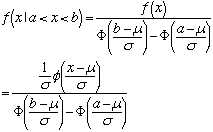
Regression with Truncated DataTruncated data occurs when some observations are not included in the analysis because of the value of the variable, that is, the sample is drawn from a restricted part of the populations. Truncation is a characteristic of the distribution from which the sample data are drawn. If x has a normal distribution with mean μ and standard deviation σ, then the density of the truncated normal distribution is
Compared with the mean of an untruncated variable, the mean of the truncated variable is greater if the truncation is from below, and is smaller if the truncation is from above. Furthermore, truncation reduces the variance compared with the variance of the untruncated distribution.
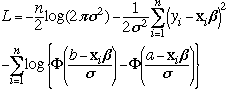
The log likelihood when a is the lower limit and b is the upper limit is
truncreg jobcen0 fem phd ment fel art cit, ll(1)
(note: 99 obs. truncated)

Truncated regression
Limit:   lower =          1                             Number of obs =    309
         upper =       +inf                             Wald chi2(6)  =  71.13
Log likelihood = -318.66024                             Prob > chi2   = 0.0000

------------------------------------------------------------------------------
     jobcen0 |      Coef.   Std. Err.      z    P>|z|     [95% Conf. Interval]
-------------+----------------------------------------------------------------
eq1          |
         fem |    .114156    .095124     1.20   0.230    -.0722837    .3005956
         phd |   .3413744   .0539561     6.33   0.000     .2356224    .4471263
        ment |   .0008171   .0006589     1.24   0.215    -.0004743    .0021085
         fel |   .1709118   .1011169     1.69   0.091    -.0272737    .3690974
         art |   .0072712   .0271957     0.27   0.789    -.0460314    .0605738
         cit |   .0021862    .001788     1.22   0.221    -.0013182    .0056905
       _cons |   1.187784   .1962769     6.05   0.000     .8030885     1.57248
-------------+----------------------------------------------------------------
sigma        |
       _cons |   .7379857   .0353198    20.89   0.000     .6687602    .8072112
------------------------------------------------------------------------------
Next, we will analysis the dataset, acadindx, that was used in the previous section. If acadindx
is no longer loaded in memory you can obtain it with the following use command.
use http://www.gseis.ucla.edu/courses/data/acadindx2
(max possible on acadindx is 200)
Let's imagine that in order to get into a special honors program, students need to score at least 165 on acadindx. So we will drop all observations in which the value of acadindx is less than 165.
drop if acadindx<165
(53 observations deleted)
Now, let's estimate the same model that we used in the section on censored data, only this time we will pretend that a 200 for acadindx is not censored.
regress acadindx female reading writing

      Source |       SS       df       MS              Number of obs =     147
-------------+------------------------------           F(  3,   143) =   35.17
       Model |  7418.94448     3  2472.98149           Prob > F      =  0.0000
    Residual |  10053.7222   143  70.3057495           R-squared     =  0.4246
-------------+------------------------------           Adj R-squared =  0.4125
       Total |  17472.6667   146  119.675799           Root MSE      =  8.3849

------------------------------------------------------------------------------
    acadindx |      Coef.   Std. Err.      t    P>|t|     [95% Conf. Interval]
-------------+----------------------------------------------------------------
      female |  -5.081622   1.491473    -3.41   0.001    -8.029805    -2.13344
     reading |   .4263403   .0874548     4.87   0.000      .253469    .5992115
     writing |   .5426893   .1062605     5.11   0.000     .3326451    .7527336
       _cons |   132.9936    5.43257    24.48   0.000     122.2551    143.7322
------------------------------------------------------------------------------
It is clear that the estimates of the coefficients are distorted due to the fact that 53 observations
are no longer in the dataset. This amounts to restriction of range on both the response variable
and the predictor variables. What this means is that if our goal is to find the relation between
adadindx and the predictor variables in the popultions, then the truncation of acadindx in our
sample is going to lead to baised estimates. A better approach to analyzing these data is to use
truncated regression. In Stata this can be accomplished using the truncreg command where the ll
option is used to indicate the lower limit of acadindx scores used in the truncation.
truncreg acadindx female reading writing, ll(165)
(note: 3 obs. truncated)

Truncated regression
Limit:   lower =        165                             Number of obs =    144
         upper =       +inf                             Wald chi2(3)  =  80.80
Log likelihood = -499.72027                             Prob > chi2   = 0.0000

------------------------------------------------------------------------------
    acadindx |      Coef.   Std. Err.      z    P>|z|     [95% Conf. Interval]
-------------+----------------------------------------------------------------
eq1          |
      female |  -5.264574   1.697022    -3.10   0.002    -8.590676   -1.938472
     reading |   .4429962   .1024458     4.32   0.000     .2422061    .6437862
     writing |   .6816854   .1324375     5.15   0.000     .4221128    .9412581
       _cons |   123.6204   7.371454    16.77   0.000     109.1726    138.0681
-------------+----------------------------------------------------------------
sigma        |
       _cons |   8.817696    .625297    14.10   0.000     7.592136    10.04326
------------------------------------------------------------------------------
The coefficients from the truncreg command differ from the OLS and represent an attempt to adjust
the analysis for the arbitrary cutoff of acadindx scores at 165.
Categorical Data Analysis Course
Phil Ender