
By now you are familiar with OLS regression, a least squares criterion is not the only way to do regression. We could look at the absolute deviations from some point estimate, say the median. We would be trying to obtain the minimum absolute deviations (MAD).
According to Koenker (2000), quantile regression is a statistical technique intended to estimate and conduct inference about conditional quantile functions. Quantile regression methods offer a mechanism for estimationg the conditional median function in addtion to other conditional quantile functions. Ordinary least squares regression asks the question "How does the conditional mean of Y depend on the covariates X?" Quantile regression asks this question at each quantile of the conditional distribution giving a more complete description of how the conditional distribution of Y given X.
In Stata this can be done using the qreg command. Here are some quantile regressions using the hsb2 dataset.
use http://www.gseis.ucla.edu/courses/data/hsb2, clear
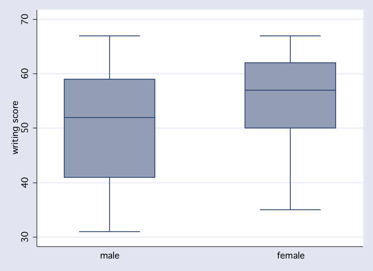
tabstat write, by(female) stat(n p25 p50 p75)
Summary for variables: write
by categories of: female
female | N p25 p50 p75
-------+----------------------------------------
male | 91 41 52 59
female | 109 50 57 62
-------+----------------------------------------
Total | 200 45.5 54 60
------------------------------------------------
graph box write, over(female)
 qreg write female, quan(.25) nolog
.25 Quantile regression Number of obs = 200
Raw sum of deviations 1333.5 (about 45)
Min sum of deviations 1243 Pseudo R2 = 0.0679
------------------------------------------------------------------------------
write | Coef. Std. Err. t P>|t| [95% Conf. Interval]
-------------+----------------------------------------------------------------
female | 9 1.797523 5.01 0.000 5.455253 12.54475
_cons | 41 1.287262 31.85 0.000 38.4615 43.5385
------------------------------------------------------------------------------
qreg write female, quan(.50) nolog
Median regression Number of obs = 200
Raw sum of deviations 1571 (about 54)
Min sum of deviations 1536 Pseudo R2 = 0.0223
------------------------------------------------------------------------------
write | Coef. Std. Err. t P>|t| [95% Conf. Interval]
-------------+----------------------------------------------------------------
female | 5 2.611711 1.91 0.057 -.1503393 10.15034
_cons | 52 1.927268 26.98 0.000 48.19939 55.80061
------------------------------------------------------------------------------
qreg write female, quan(.75) nolog
.75 Quantile regression Number of obs = 200
Raw sum of deviations 1084.5 (about 60)
Min sum of deviations 1060 Pseudo R2 = 0.0226
------------------------------------------------------------------------------
write | Coef. Std. Err. t P>|t| [95% Conf. Interval]
-------------+----------------------------------------------------------------
female | 3 1.23163 2.44 0.016 .5712036 5.428796
_cons | 59 .9385943 62.86 0.000 57.14908 60.85092
------------------------------------------------------------------------------
list write in 10/14
+-------+
| write |
|-------|
10. | 55 |
11. | 46 |
12. | 65 |
13. | 60 |
14. | 63 |
+-------+
replace write = 600 in 13
(1 real change made)
qreg write female, quan(.5) nolog
Median regression Number of obs = 200
Raw sum of deviations 2111 (about 54)
Min sum of deviations 2076 Pseudo R2 = 0.0166
------------------------------------------------------------------------------
write | Coef. Std. Err. t P>|t| [95% Conf. Interval]
-------------+----------------------------------------------------------------
female | 5 2.611711 1.91 0.057 -.1503393 10.15034
_cons | 52 1.927268 26.98 0.000 48.19939 55.80061
------------------------------------------------------------------------------
replace write = 6000 in 13
(1 real change made)
qreg write female, quan(.5) nolog
Median regression Number of obs = 200
Raw sum of deviations 7511 (about 54)
Min sum of deviations 7476 Pseudo R2 = 0.0047
------------------------------------------------------------------------------
write | Coef. Std. Err. t P>|t| [95% Conf. Interval]
-------------+----------------------------------------------------------------
female | 5 2.611711 1.91 0.057 -.1503393 10.15034
_cons | 52 1.927268 26.98 0.000 48.19939 55.80061
------------------------------------------------------------------------------
replace write =6000 if write>=60
(52 real changes made)
qreg write female, quan(.5) nolog
Median regression Number of obs = 200
Raw sum of deviations 316210 (about 54)
Min sum of deviations 316175 Pseudo R2 = 0.0001
------------------------------------------------------------------------------
write | Coef. Std. Err. t P>|t| [95% Conf. Interval]
-------------+----------------------------------------------------------------
female | 5 2.611711 1.91 0.057 -.1503393 10.15034
_cons | 52 1.927268 26.98 0.000 48.19939 55.80061
------------------------------------------------------------------------------
univar write
-------------- Quantiles --------------
Variable n Mean S.D. Min .25 Mdn .75 Max
-------------------------------------------------------------------------------
write 200 1625.97 2633.00 31.00 45.50 54.00 6000.00 6000.00
-------------------------------------------------------------------------------
qreg write female, quan(.25) nolog
.25 Quantile regression Number of obs = 200
Raw sum of deviations 1333.5 (about 45)
Min sum of deviations 1243 Pseudo R2 = 0.0679
------------------------------------------------------------------------------
write | Coef. Std. Err. t P>|t| [95% Conf. Interval]
-------------+----------------------------------------------------------------
female | 9 1.797523 5.01 0.000 5.455253 12.54475
_cons | 41 1.287262 31.85 0.000 38.4615 43.5385
------------------------------------------------------------------------------
qreg write female, quan(.50) nolog
Median regression Number of obs = 200
Raw sum of deviations 1571 (about 54)
Min sum of deviations 1536 Pseudo R2 = 0.0223
------------------------------------------------------------------------------
write | Coef. Std. Err. t P>|t| [95% Conf. Interval]
-------------+----------------------------------------------------------------
female | 5 2.611711 1.91 0.057 -.1503393 10.15034
_cons | 52 1.927268 26.98 0.000 48.19939 55.80061
------------------------------------------------------------------------------
qreg write female, quan(.75) nolog
.75 Quantile regression Number of obs = 200
Raw sum of deviations 1084.5 (about 60)
Min sum of deviations 1060 Pseudo R2 = 0.0226
------------------------------------------------------------------------------
write | Coef. Std. Err. t P>|t| [95% Conf. Interval]
-------------+----------------------------------------------------------------
female | 3 1.23163 2.44 0.016 .5712036 5.428796
_cons | 59 .9385943 62.86 0.000 57.14908 60.85092
------------------------------------------------------------------------------
list write in 10/14
+-------+
| write |
|-------|
10. | 55 |
11. | 46 |
12. | 65 |
13. | 60 |
14. | 63 |
+-------+
replace write = 600 in 13
(1 real change made)
qreg write female, quan(.5) nolog
Median regression Number of obs = 200
Raw sum of deviations 2111 (about 54)
Min sum of deviations 2076 Pseudo R2 = 0.0166
------------------------------------------------------------------------------
write | Coef. Std. Err. t P>|t| [95% Conf. Interval]
-------------+----------------------------------------------------------------
female | 5 2.611711 1.91 0.057 -.1503393 10.15034
_cons | 52 1.927268 26.98 0.000 48.19939 55.80061
------------------------------------------------------------------------------
replace write = 6000 in 13
(1 real change made)
qreg write female, quan(.5) nolog
Median regression Number of obs = 200
Raw sum of deviations 7511 (about 54)
Min sum of deviations 7476 Pseudo R2 = 0.0047
------------------------------------------------------------------------------
write | Coef. Std. Err. t P>|t| [95% Conf. Interval]
-------------+----------------------------------------------------------------
female | 5 2.611711 1.91 0.057 -.1503393 10.15034
_cons | 52 1.927268 26.98 0.000 48.19939 55.80061
------------------------------------------------------------------------------
replace write =6000 if write>=60
(52 real changes made)
qreg write female, quan(.5) nolog
Median regression Number of obs = 200
Raw sum of deviations 316210 (about 54)
Min sum of deviations 316175 Pseudo R2 = 0.0001
------------------------------------------------------------------------------
write | Coef. Std. Err. t P>|t| [95% Conf. Interval]
-------------+----------------------------------------------------------------
female | 5 2.611711 1.91 0.057 -.1503393 10.15034
_cons | 52 1.927268 26.98 0.000 48.19939 55.80061
------------------------------------------------------------------------------
univar write
-------------- Quantiles --------------
Variable n Mean S.D. Min .25 Mdn .75 Max
-------------------------------------------------------------------------------
write 200 1625.97 2633.00 31.00 45.50 54.00 6000.00 6000.00
-------------------------------------------------------------------------------
Note that increasing values greater than the median did not change the coefficients for the median
regression.
We need to reload the data because of the changes that were made.
use http://www.gseis.ucla.edu/courses/data/hsb2, clear

tabstat write, by(prog) stat(n p25 median p75)

Summary for variables: write
     by categories of: prog (type of program)

    prog |         N       p25       p50       p75
---------+----------------------------------------
 general |        45        44        54        59
academic |       105        52        59        62
vocation |        50        40        46        54
---------+----------------------------------------
   Total |       200      45.5        54        60
--------------------------------------------------

sort prog
graph write, box by(prog)


xi: qreg write i.prog, quant(.50) nolog
i.prog            _Iprog_1-3          (naturally coded; _Iprog_1 omitted)

Median regression                                    Number of obs =       200
  Raw sum of deviations     1571 (about 54)
  Min sum of deviations     1364                     Pseudo R2     =    0.1318

------------------------------------------------------------------------------
       write |      Coef.   Std. Err.      t    P>|t|     [95% Conf. Interval]
-------------+----------------------------------------------------------------
    _Iprog_2 |          5   1.955055     2.56   0.011     1.144477    8.855523
    _Iprog_3 |         -8   2.302537    -3.47   0.001    -12.54079   -3.459214
       _cons |         54   1.646609    32.79   0.000     50.75276    57.24724
------------------------------------------------------------------------------

test _Iprog_2 _Iprog_3

 ( 1)  _Iprog_2 = 0.0
 ( 2)  _Iprog_3 = 0.0

       F(  2,   197) =   23.00
            Prob > F =    0.0000

xi: qreg write i.prog, quant(.25) nolog
i.prog            _Iprog_1-3          (naturally coded; _Iprog_1 omitted)

.25 Quantile regression                              Number of obs =       200
  Raw sum of deviations   1333.5 (about 45)
  Min sum of deviations   1159.5                     Pseudo R2     =    0.1305

------------------------------------------------------------------------------
       write |      Coef.   Std. Err.      t    P>|t|     [95% Conf. Interval]
-------------+----------------------------------------------------------------
    _Iprog_2 |          8   2.717471     2.94   0.004     2.640933    13.35907
    _Iprog_3 |         -4   3.262362    -1.23   0.222    -10.43364    2.433635
       _cons |         44   2.229953    19.73   0.000     39.60236    48.39764
------------------------------------------------------------------------------

test _Iprog_2 _Iprog_3

 ( 1)  _Iprog_2 = 0.0
 ( 2)  _Iprog_3 = 0.0

       F(  2,   197) =   10.37
            Prob > F =    0.0000

xi: qreg write i.prog, quant(.75) nolog
i.prog            _Iprog_1-3          (naturally coded; _Iprog_1 omitted)

.75 Quantile regression                              Number of obs =       200
  Raw sum of deviations   1084.5 (about 60)
  Min sum of deviations      993                     Pseudo R2     =    0.0844

------------------------------------------------------------------------------
       write |      Coef.   Std. Err.      t    P>|t|     [95% Conf. Interval]
-------------+----------------------------------------------------------------
    _Iprog_2 |          3   1.576171     1.90   0.058    -.1083338    6.108334
    _Iprog_3 |         -5   1.888316    -2.65   0.009    -8.723908   -1.276092
       _cons |         59   1.284961    45.92   0.000     56.46595    61.53405
------------------------------------------------------------------------------

test _Iprog_2 _Iprog_3

 ( 1)  _Iprog_2 = 0.0
 ( 2)  _Iprog_3 = 0.0

       F(  2,   197) =   11.72
            Prob > F =    0.0000

We have been using dummy (indicator) coding for the categorical variable.  There are other possible codings that
we could use.  For this example, I would like to use a coding that compares general with vocational
and one that compares the average of general and vocational with academic.  We can create the
coding using variable characteristics in Stata and apply them to the model using the xi3
command available for ATS via the Internet.
xi: qreg write i.prog, quant(.50) nolog
i.prog _Iprog_1-3 (naturally coded; _Iprog_1 omitted)
Median regression Number of obs = 200
Raw sum of deviations 1571 (about 54)
Min sum of deviations 1364 Pseudo R2 = 0.1318
------------------------------------------------------------------------------
write | Coef. Std. Err. t P>|t| [95% Conf. Interval]
-------------+----------------------------------------------------------------
_Iprog_2 | 5 1.955055 2.56 0.011 1.144477 8.855523
_Iprog_3 | -8 2.302537 -3.47 0.001 -12.54079 -3.459214
_cons | 54 1.646609 32.79 0.000 50.75276 57.24724
------------------------------------------------------------------------------
test _Iprog_2 _Iprog_3
( 1) _Iprog_2 = 0.0
( 2) _Iprog_3 = 0.0
F( 2, 197) = 23.00
Prob > F = 0.0000
xi: qreg write i.prog, quant(.25) nolog
i.prog _Iprog_1-3 (naturally coded; _Iprog_1 omitted)
.25 Quantile regression Number of obs = 200
Raw sum of deviations 1333.5 (about 45)
Min sum of deviations 1159.5 Pseudo R2 = 0.1305
------------------------------------------------------------------------------
write | Coef. Std. Err. t P>|t| [95% Conf. Interval]
-------------+----------------------------------------------------------------
_Iprog_2 | 8 2.717471 2.94 0.004 2.640933 13.35907
_Iprog_3 | -4 3.262362 -1.23 0.222 -10.43364 2.433635
_cons | 44 2.229953 19.73 0.000 39.60236 48.39764
------------------------------------------------------------------------------
test _Iprog_2 _Iprog_3
( 1) _Iprog_2 = 0.0
( 2) _Iprog_3 = 0.0
F( 2, 197) = 10.37
Prob > F = 0.0000
xi: qreg write i.prog, quant(.75) nolog
i.prog _Iprog_1-3 (naturally coded; _Iprog_1 omitted)
.75 Quantile regression Number of obs = 200
Raw sum of deviations 1084.5 (about 60)
Min sum of deviations 993 Pseudo R2 = 0.0844
------------------------------------------------------------------------------
write | Coef. Std. Err. t P>|t| [95% Conf. Interval]
-------------+----------------------------------------------------------------
_Iprog_2 | 3 1.576171 1.90 0.058 -.1083338 6.108334
_Iprog_3 | -5 1.888316 -2.65 0.009 -8.723908 -1.276092
_cons | 59 1.284961 45.92 0.000 56.46595 61.53405
------------------------------------------------------------------------------
test _Iprog_2 _Iprog_3
( 1) _Iprog_2 = 0.0
( 2) _Iprog_3 = 0.0
F( 2, 197) = 11.72
Prob > F = 0.0000
We have been using dummy (indicator) coding for the categorical variable. There are other possible codings that
we could use. For this example, I would like to use a coding that compares general with vocational
and one that compares the average of general and vocational with academic. We can create the
coding using variable characteristics in Stata and apply them to the model using the xi3
command available for ATS via the Internet.
findit xi3

char prog[user] (1 0 -1 \ -.5 1 -.5)

xi3: qreg write u.prog, nolog
u.prog            _Iprog_1-3          (naturally coded; _Iprog_3 omitted)

Median regression                                    Number of obs =       200
  Raw sum of deviations     1571 (about 54)
  Min sum of deviations     1364                     Pseudo R2     =    0.1318

------------------------------------------------------------------------------
       write |      Coef.   Std. Err.      t    P>|t|     [95% Conf. Interval]
-------------+----------------------------------------------------------------
    _Iprog_1 |          8   2.302537     3.47   0.001     3.459214    12.54079
    _Iprog_2 |          9   1.560877     5.77   0.000     5.921826    12.07817
       _cons |         53   .8441035    62.79   0.000     51.33536    54.66464
------------------------------------------------------------------------------
In this next series of analyses we will
look at models which include an interaction. We will use the variables female and
socst and create an interaction fxs.
generate fxs = female*socst

qreg write female socst fxs, quant(.50) nolog

Median regression                                    Number of obs =       200
  Raw sum of deviations     1571 (about 54)
  Min sum of deviations 1170.167                     Pseudo R2     =    0.2551

------------------------------------------------------------------------------
       write |      Coef.   Std. Err.      t    P>|t|     [95% Conf. Interval]
-------------+----------------------------------------------------------------
      female |       13.5    11.8569     1.14   0.256    -9.883489    36.88349
       socst |   .6666667   .1567594     4.25   0.000      .357515    .9758183
         fxs |  -.1666667   .2210759    -0.75   0.452    -.6026596    .2693262
       _cons |         15   8.357237     1.79   0.074    -1.481651    31.48165
------------------------------------------------------------------------------

qreg write female socst fxs, quant(.25) nolog

.25 Quantile regression                              Number of obs =       200
  Raw sum of deviations   1333.5 (about 45)
  Min sum of deviations      895                     Pseudo R2     =    0.3288

------------------------------------------------------------------------------
       write |      Coef.   Std. Err.      t    P>|t|     [95% Conf. Interval]
-------------+----------------------------------------------------------------
      female |        9.1   5.512101     1.65   0.100    -1.770642    19.97064
       socst |         .7   .0696054    10.06   0.000     .5627283    .8372717
         fxs |        -.1   .1014278    -0.99   0.325    -.3000299    .1000299
       _cons |        9.3   3.770638     2.47   0.015     1.863769    16.73623
------------------------------------------------------------------------------

qreg write female socst fxs, quant(.75) nolog

.75 Quantile regression                              Number of obs =       200
  Raw sum of deviations   1084.5 (about 60)
  Min sum of deviations 866.3857                     Pseudo R2     =    0.2011

------------------------------------------------------------------------------
       write |      Coef.   Std. Err.      t    P>|t|     [95% Conf. Interval]
-------------+----------------------------------------------------------------
      female |   20.31428   5.465128     3.72   0.000     9.536281    31.09229
       socst |         .6   .0689976     8.70   0.000     .4639269    .7360731
         fxs |  -.3142857   .1016025    -3.09   0.002    -.5146602   -.1139111
       _cons |       24.4   3.647607     6.69   0.000      17.2064     31.5936
------------------------------------------------------------------------------
Next, we will take a look at the same model using an alternative coding scheme
involving the difference between the groups and the grand median.
xi3: qreg write e.female*socst, quan(.5) nolog
d.female          _Ifemale_0-1        (naturally coded; _Ifemale_0 omitted)
d.female*socst    _IfemXsocst_#       (coded as above)

Median regression                                    Number of obs =       200
  Raw sum of deviations     1571 (about 54)
  Min sum of deviations 1170.167                     Pseudo R2     =    0.2551

------------------------------------------------------------------------------
       write |      Coef.   Std. Err.      t    P>|t|     [95% Conf. Interval]
-------------+----------------------------------------------------------------
  _Ifemale_1 |       6.75   5.928452     1.14   0.256    -4.941744    18.44174
       socst |   .5833333    .110538     5.28   0.000     .3653369    .8013298
_IfemXsocs~1 |  -.0833333    .110538    -0.75   0.452    -.3013298    .1346631
       _cons |      21.75   5.928452     3.67   0.000     10.05826    33.44174
------------------------------------------------------------------------------

describe _Ifemale_1

              storage  display     value
variable name   type   format      label      variable label
-------------------------------------------------------------------------------
_Ifemale_1      byte   %8.0g                  female(1 vs. grand mean)

tabulate _Ifemale_1

   female(1 |
  vs. grand |
      mean) |      Freq.     Percent        Cum.
------------+-----------------------------------
         -1 |         91       45.50       45.50
          1 |        109       54.50      100.00
------------+-----------------------------------
      Total |        200      100.00

xi3: qreg write e.female*socst, quan(.25) nolog
d.female          _Ifemale_0-1        (naturally coded; _Ifemale_0 omitted)
d.female*socst    _IfemXsocst_#       (coded as above)

.25 Quantile regression                              Number of obs =       200
  Raw sum of deviations   1333.5 (about 45)
  Min sum of deviations      895                     Pseudo R2     =    0.3288

------------------------------------------------------------------------------
       write |      Coef.   Std. Err.      t    P>|t|     [95% Conf. Interval]
-------------+----------------------------------------------------------------
  _Ifemale_1 |       4.55   2.756051     1.65   0.100     -.885321    9.985321
       socst |        .65   .0507139    12.82   0.000     .5499851    .7500149
_IfemXsocs~1 |       -.05   .0507139    -0.99   0.325    -.1500149    .0500149
       _cons |      13.85   2.756051     5.03   0.000     8.414679    19.28532
------------------------------------------------------------------------------

xi3: qreg write 3.female*socst, quan(.75) nolog
d.female          _Ifemale_0-1        (naturally coded; _Ifemale_0 omitted)
d.female*socst    _IfemXsocst_#       (coded as above)

.75 Quantile regression                              Number of obs =       200
  Raw sum of deviations   1084.5 (about 60)
  Min sum of deviations 866.3857                     Pseudo R2     =    0.2011

------------------------------------------------------------------------------
       write |      Coef.   Std. Err.      t    P>|t|     [95% Conf. Interval]
-------------+----------------------------------------------------------------
  _Ifemale_1 |   10.15714   2.732564     3.72   0.000      4.76814    15.54614
       socst |   .4428572   .0508013     8.72   0.000     .3426699    .5430444
_IfemXsocs~1 |  -.1571428   .0508013    -3.09   0.002    -.2573301   -.0569556
       _cons |   34.55714   2.732564    12.65   0.000     29.16814    39.94614
------------------------------------------------------------------------------
Categorical Data Analysis Course
Phil Ender -- 5/15/04